Code
library(tidyverse)
library(readxl)
library(lubridate)
knitr::opts_chunk$set(echo = TRUE, warning=FALSE, message=FALSE)library(tidyverse)
library(readxl)
library(lubridate)
knitr::opts_chunk$set(echo = TRUE, warning=FALSE, message=FALSE)The Internet Movie Database or IMDb (imdb.com) is an extensive collection of information about movies and TV shows from around the world. It was founded in 1990 but contains information about film titles from all time periods. This information is gathered by IMDb employees but also largely contributed to by external parties. IMDb states “while [they] actively gather information from and verify items with studios and filmmakers, the bulk of [their] information is submitted by people in the industry and visitors” (“Where Does”). One of the more unique features of the database is that the website allows registered users (anybody with a free IMDb account) to rate film titles on a scale of 1 to 10. IMDb then aggregates a score for these titles using all user ratings as input to an undefined weighted average algorithm. Each title that has at least one user rating then contains an IMDb rating (for example, the first episode of the series Game of Thrones, Winter is Coming, is rated 8.9).
Along with their standard website, IMDb provides free access to non-commercial data sets at developer.imdb.com/non-commercial-datasets, which contain information about all of the titles maintained by the database. The data sets are updated daily and in this project the data is up to date to June 13, 2023. The intention of this project is to use these data sets to perform analysis on TV series episode titles by exploring their user ratings. There are three data set files that contain information pertaining to this task. The title.basics.tsv file contains data about all the titles on IMDb including movies, TV series, individual TV episodes, shorts, etc. The title.episode.tsv file maps TV episode titles to their parent TV series title, and also includes the season and episode number. The title.ratings.tsv file contains the rating for each title. Using these files we are able to create visualizations and generate statistics that reveal interesting trends among the data.
Let’s read in the title.basics.tsv data and examine the rows
title_basics <- read_tsv("noah_data/title.basics.tsv")
title_basicsdim(title_basics)[1] 9926879 9As we can see the data frame is very large (over 9 million rows). However, the data we will actually use for analysis will be much less after cleaning. Each row in the data frame represents one “title” (could be a movie, TV series, individual TV episode, short, etc.). A description of each of the data columns is as follows:
- tconst: alphanumeric unique identifier of the title
- titleType: the type/format of the title (e.g. movie, short, TV series, TV episode, video, etc.)
- primaryTitle: the more popular title / the title used by the filmmakers on promotional materials at the point of release
- originalTitle: original title, in the original language
- isAdult: 0: non-adult title; 1: adult title
- startYear: represents the release year of a title. In the case of TV Series, it is the series start year
- endYear: TV Series end year. “Backslash N” for all other title types
- runtimeMinutes: primary runtime of the title, in minutes
- genres: includes up to three genres associated with the title
The code below reveals the data types of the data columns.
spec(title_basics)cols(
tconst = col_character(),
titleType = col_character(),
primaryTitle = col_character(),
originalTitle = col_character(),
isAdult = col_double(),
startYear = col_character(),
endYear = col_character(),
runtimeMinutes = col_character(),
genres = col_character()
)Similarly, lets read in and describe the title.episode.tsv file.
title_episode <- read_tsv("noah_data/title.episode.tsv")
title_episodedim(title_episode)[1] 7545323 4A description of each of the data columns in this data frame is as follows:
- tconst: alphanumeric identifier of episode
- parentTconst: alphanumeric identifier of the parent TV Series
- seasonNumber: season number the episode belongs to
- episodeNumber: episode number of the tconst in the TV series
The code below reveals the data types of the data columns.
spec(title_episode)cols(
tconst = col_character(),
parentTconst = col_character(),
seasonNumber = col_character(),
episodeNumber = col_character()
)Finally, lets read in and describe the title.ratings.tsv file.
title_ratings <- read_tsv("noah_data/title.ratings.tsv")
title_ratingsdim(title_ratings)[1] 1318736 3A description of each of the data columns in this data frame is as follows:
- tconst: alphanumeric identifier of episode
- averageRating: weighted average of all the individual user ratings
- numVotes: number of rating votes the title has received
The code below reveals the data types of the data columns.
spec(title_ratings)cols(
tconst = col_character(),
averageRating = col_double(),
numVotes = col_double()
)The goal of the data tidying will be to consolidate the information from the three data files into two data frames that can be used for analysis. Each case in the data frames should represent an episode of a TV series. The data frames will have columns that include the episodes average viewer rating, number of rated votes, the name and identifier of the series the episode belongs to, and the season and episode numbers. The difference between the two data frames will be that one will contain all TV series episodes in the data set, and the other will only contain episodes that belong to series which have all episodes rated by viewers (no NA values).
First, we will drop all non TV Episodes from the title_basics data frame to get a data frame of all titles that are TV episodes. We will also remove adult TV episodes.
episodes_all <- subset(title_basics, titleType == "tvEpisode" & isAdult == 0)
episodes_allNext we will perform a left outer join between the episodes data frame and the title_ratings data frame to add the rating and the number of votes to the episodes data frame.
episodes_all <- left_join(episodes_all, title_ratings, by = "tconst")
episodes_allNow we will perform another left outer join between the episodes data frame and the title_episode data frame, to add the parent TV series identifier, the season number, and episode number to the episode data frame.
episodes_all <- left_join(episodes_all, title_episode, by = "tconst")
episodes_allNow lets add the series title to each episode case.
episodes_all <- episodes_all %>%
left_join(title_basics %>% select(tconst, primaryTitle), by = c("parentTconst" = "tconst"))
episodes_allLets now clean up the data by renaming columns and removing columns we don’t need. In particular we will remove the titleType column since it is always “tvEpisode”, the originalTitle column since the primaryTitle column is sufficient, the isAdult column since it is always 0, and the endYear column since we are not concerned with when a show ended. We will use the number of episodes, seasons, and run times to compare shows by length.
episodes_all <- select(episodes_all, seriesID = parentTconst, seriesName = primaryTitle.y, episodeID = tconst, episodeName = primaryTitle.x, startYear, runtimeMinutes, genres, averageRating, numVotes, seasonNumber, episodeNumber)
episodes_allFinally, lets change the numerical columns to integers rather than chars, change the startYear column to a date format, and remove dates outside the range 1940-2022.
episodes_all <- mutate(episodes_all, startYear = as.Date(paste0(startYear, "-01-01"), format = "%Y-%m-%d"), runtimeMinutes = as.integer(runtimeMinutes), seasonNumber = as.integer(seasonNumber), episodeNumber = as.integer(episodeNumber)) %>%
filter(startYear < as.Date("2023-01-01") & startYear > as.Date("1939-01-01"))
episodes_allThe data frame is now tidied, with each case representing an episode of a TV series. However, not all of the TV series episodes have an average rating (several rows have NA for this column). It will be helpful in our analysis to have access to a data frame that contains only the episodes that belong to series for which all episodes have a rating. In order to make this data frame, first we need to make a set of all the series identifiers (seriesID) that have at least one episode with no ratings.
unrated_series <- unique(episodes_all$seriesID[is.na(episodes_all$averageRating)])
length(unrated_series)[1] 159049There are 159,049 series with at least one episode that is unrated. Now, we will remove all episodes of these series and store the result in a new data frame.
episodes_rated <- subset(episodes_all, !(seriesID %in% unrated_series))
episodes_ratedWe now have two tidied data frames for analysis. The episodes_all data frame contains all TV series episodes, while the episodes_rated data frame contains all of the TV series episodes that have a rating and belong to a TV series with each episode rated. Each column in both data frames is labeled appropriately with a descriptive name and the data types make sense for this data set. A final description of the data in each column of the two data frames is:
- seriesID: a unique identifier for the TV series
- seriesName: the name of the series
- episodeID: a unique identifier for the series episode
- episodeName: the name of the episode
- startYear: the year the series started
- runtimeMinutesv: the runtime of the series in minutes
- averageRating: the average viewer rating of the episode
- numVotes: the number of rating votes the episode received
- seasonNumber: the number of the season
- episodeNumber: the number of the episode
A few research questions that will be answered with this data set are:
1. How have viewers ratings of TV series episodes and the quantity of TV series episodes released per year changed over time?
2. How has the number of episodes produced varied over time for the different genres in the dataset? Does this correlate with user ratings for specific genres?
3. Does a longer TV series indicate a higher rated series by viewers?
In order to examine how TV series episodes have evolved over time in terms of viewer ratings, we can group TV series episodes by their startYear (year when the episode aired). We can then compute the average rating of all episodes that aired this year. In order to examine how the quantity of new TV series episodes aired has changed over the years, we can also as computer the count of all episodes that aired each year.
quantity_quality <- episodes_all %>%
select(startYear, averageRating) %>%
group_by(startYear) %>%
summarise(averageRating = mean(averageRating, na.rm = TRUE), totalEpisodes = n())
quantity_qualityFrom the output we can see that the average viewer rating of all TV series episodes has remained fairly constant from 1948-2023 at around 7.0-7.5. However, it is evident that the number of TV series episodes produced per year has increased each year. We can plot these results to better understand the trends of quantity and quality of TV series episodes over time.
ggplot(quantity_quality, aes(x = startYear, y = averageRating)) +
geom_line(color = "red", linewidth = 1) +
theme_minimal() +
labs(title = "Average TV Series Episode Viewer Rating vs Time", x = "Year", y = "Average Viewer Rating") +
ylim(0, 10)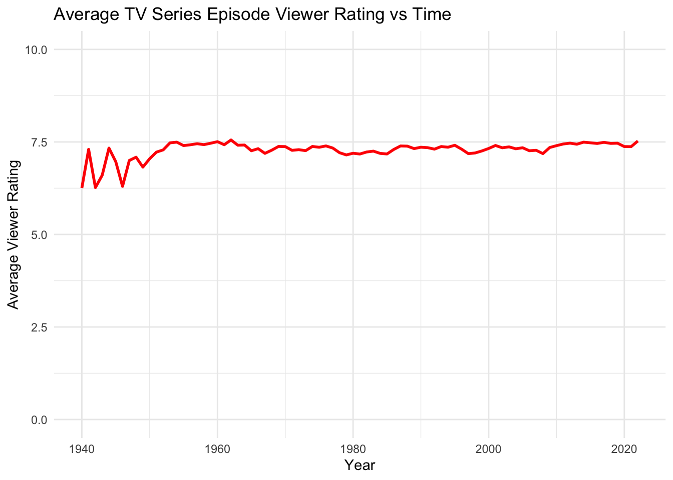
ggplot(quantity_quality, aes(x = startYear, y = totalEpisodes)) +
geom_line(color = "blue", linewidth = 1) +
theme_minimal() +
labs(title = "Number of New Episodes Aired vs Time", x = "Year", y = "Number of Episodes")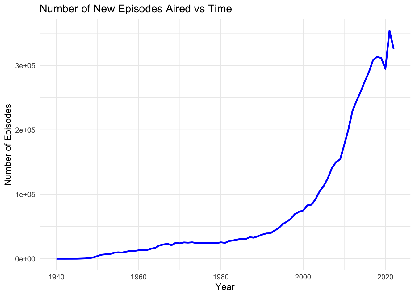
From the Average Viewer Rating vs Time graph above we can confirm our previous observation that the average TV series episodes rating has remained fairly constant from 1940-2022. There appears to be some larger variations among the years between 1940 and 1950, however this is likely due to the fact that the sample size is much smaller (less TV episodes were released this year). This can be seen in the second graph, the Number of New Episodes Aired vs Time. In this graph it is evident that between 1940 and 2020, the number of TV series episodes has grown exponentially. We can see that the rate of change of the number of episodes produced per year jumped dramatically during the mid 2000’s. This could be due to the explosion of streaming services during this time, allowing viewers to consume series more quickly by binging them. It is also interesting to note that the amount of new episodes aired dropped in 2020, which could be due to the COVID-19 pandemic. Episode production likely slowed down during this time which may have resulted in several seasons or individual episodes moving back their release dates.
One underlying factor of this data that could affect how viewers rate TV series is the fact that IMDb did not exist before 1990. Therefore, users of the platform were unable to rate episodes immediately after watching them for the first time before 1990. This could possibly mean that the number of ratings per TV series episode was lower prior to 1990 because casual users are more likely to rate new shows that they just watched. However, it is also possible that since there are significantly more shows overall during the 2000’s, the number of ratings per episode may have dropped if the viewer population did not increase at the same rate. In order to examine this trend, we need to create a new data frame that calculates the number of ratings per episode for each year. Then, we can plot
number_ratings <- episodes_all %>%
select(startYear, averageRating, numVotes) %>%
group_by(startYear) %>%
summarise(averageRating = mean(averageRating, na.rm = TRUE), ratingsPerEpisodes = sum(numVotes, na.rm = TRUE) / n())
number_ratingsggplot(number_ratings, aes(x = startYear, y = ratingsPerEpisodes)) +
geom_line(color = "purple", linewidth = 1) +
theme_minimal() +
labs(title = "Viewer Ratings Per TV Series Episode vs Time", x = "Year", y = "Ratings Per Episode")
From the plot we can see that there is a significant change in the number of ratings per episode after IMDb was created in 1990. This may confirm the theory that users were more likely to rate episodes as they came out rather than retroactively rating older shows. There is an outlier to this trend around 1960 when there were a few years where the number of ratings per episode approached 20 ratings per episode. This is around the average from 1990-2010. This may suggest that during this time period there were series’ that were especially popular, causing the average number of ratings to spike as a significant number users went back and rated the series in the 90’s and 2000’s.
Another trend we can see from the plot is that from 1990 onward there appears to be a steady increase in the average number of ratings per episode. This is interesting combined with the fact that the number of total episodes increased dramatically during this time, as well as the fact that the average rating of all episodes remained relatively constant. This may mean that TV series popularity increased during this time, since the number of viewer ratings per episode was able to increase along with the total number of episodes. However, it could also mean that the IMDb website grew in popularity during this time, with more users on the site rating new shows as they watched them.
In order to examine the popularity trends of genres over time, we will first split the rows so that each row only contains one genre (episodes with more than one genre will have more than one row, each representing one genre).
genre_split <- episodes_all %>%
separate_rows(genres, sep = ",")
genre_splitNow that each row only has one genre, we can group by genre to see how many genres the data set contains.
genre_count <- genre_split %>%
group_by(genres) %>%
summarise(numberOfEpisodes = n()) %>%
arrange(desc(numberOfEpisodes))
genre_countLooking through the 29 genres, we can see that some TV episodes do not have a genre listed (“\N”). We should remove this genre from the data frame before creating any visualizations.
genre_count <- subset(genre_count, genres != "\\N")
genre_countSince 28 genres is too many to plot at once, we will start by looking at the top 10 most common genres to see how they have evolved over time.
top_ten_genres <- genre_count %>%
head(10)color_palette <- c("black", "blue", "green", "cyan", "purple", "orange", "red", "magenta", "forestgreen", "brown")
genre_split %>%
group_by(genres, startYear) %>%
summarise(numberOfEpisodes = n()) %>%
filter(genres %in% top_ten_genres$genres) %>%
ggplot(aes(x = startYear, y = numberOfEpisodes, color = genres)) +
geom_line(linewidth = 1, alpha = 0.7) +
scale_color_manual(values = color_palette) +
labs(x = "Year", y = "Number of Episodes", color = "Genres") +
ggtitle("Number of New Episodes Aired per Year by Genre (Top Ten Genres)") +
theme(panel.background = element_rect(fill = "white")) +
theme(panel.grid.major = element_line(color = "gray", linetype = "dashed"))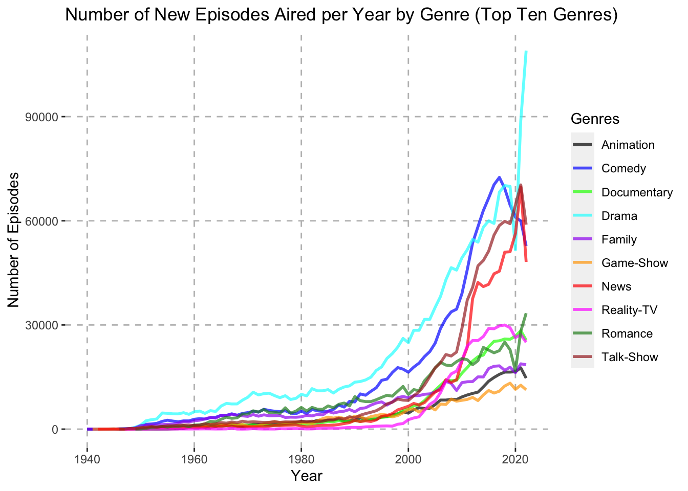
We can see from the Number of New Episodes Aired per Year by Genre graph that several genres grew substantially in terms of episode releases during the mid 2000’s, namely Drama, Comedy, Talk-Show, and News. While it is clear these genres had a sharp increase in the number of new episodes aired, it is difficult to discern whether or not these genres actually became more popular in terms of the total percentage of new shows created. Their growth during the mid 2000’s could just come as a result of more shows being produced overall. In order to tease out the growth in overall shows and only compare the genres amongst themselves, we can look at the percentage of total shows released in each year that fall under each of these genres instead.
genre_split %>%
group_by(genres, startYear) %>%
summarise(numberOfEpisodes = n()) %>%
group_by(startYear) %>%
mutate(percentage = numberOfEpisodes / sum(numberOfEpisodes) * 100) %>%
filter(genres %in% top_ten_genres$genres) %>%
ggplot(aes(x = startYear, y = percentage, color = genres)) +
geom_line(linewidth = 1, alpha = 0.7) +
scale_color_manual(values = color_palette) +
labs(x = "Year", y = "Percentage of Total Episode Count", color = "Genres") +
ggtitle("Percentage of New Episodes Aired per Year by Genre (Top Ten Genres)") +
theme(panel.background = element_rect(fill = "white")) +
theme(panel.grid.major = element_line(color = "gray", linetype = "dashed"))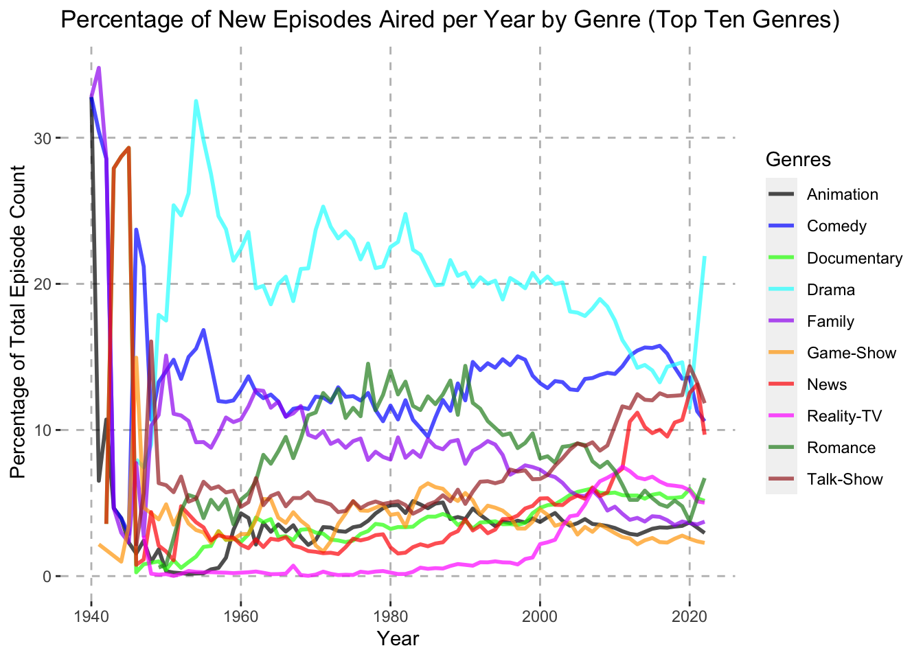
From the Percentage of New Episodes Aired per Year by Genre (Top Ten Genres) graph, we can see that Talk-Show and News genres did indeed increase during the 2000’s in terms of percentage of total new episodes aired. However, the Drama genre did not increase during the early and mid 2000’s, though it skyrocketed from 2020-2022. The Comedy genre mostly remained constant throughout the 2000’s. One of the more notable trends in this graph is Reality-TV, which made up almost none of the new episodes released until 2000. It then rose over the 2000’s to eventually make up nearly 8% of all new episode releases.
Let’s now look at the other 19 genres.
eleven_to_twenty_genres <- genre_count %>%
slice(11:20)
twenty_one_to_twenty_eight_genres <- genre_count %>%
slice(21:29)
genre_split %>%
group_by(genres, startYear) %>%
summarise(numberOfEpisodes = n()) %>%
filter(genres %in% eleven_to_twenty_genres$genres) %>%
ggplot(aes(x = startYear, y = numberOfEpisodes, color = genres)) +
geom_line(linewidth = 1, alpha = 0.7) +
scale_color_manual(values = color_palette) +
labs(x = "Year", y = "Number of Episodes", color = "Genres") +
ggtitle("Number of New Episodes Aired per Year by Genre (Genres 11-20)") +
theme(panel.background = element_rect(fill = "white")) +
theme(panel.grid.major = element_line(color = "gray", linetype = "dashed"))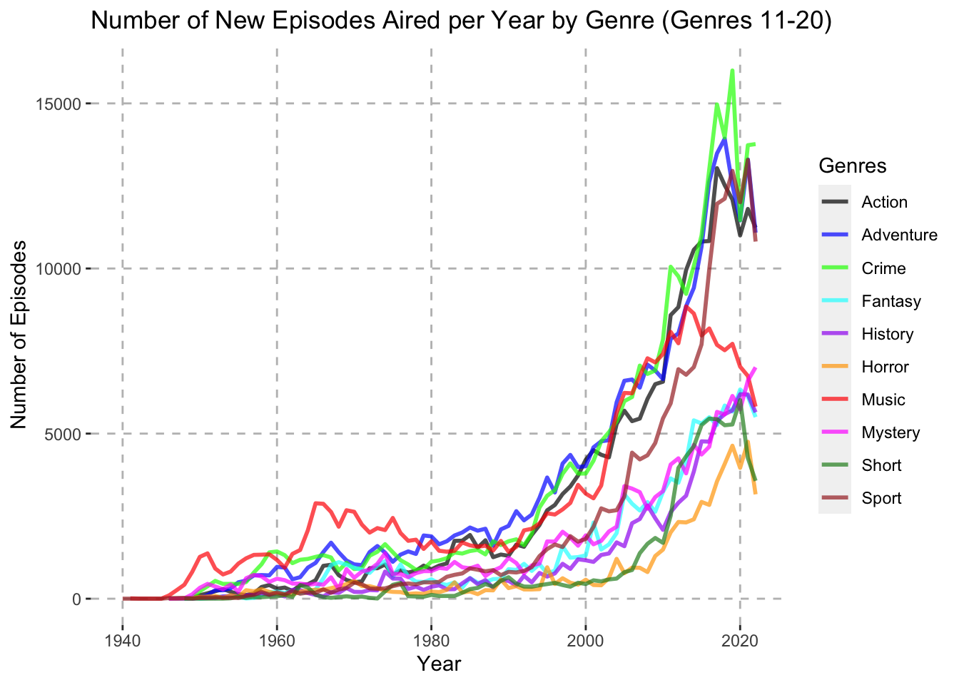
genre_split %>%
group_by(genres, startYear) %>%
summarise(numberOfEpisodes = n()) %>%
group_by(startYear) %>%
mutate(percentage = numberOfEpisodes / sum(numberOfEpisodes) * 100) %>%
filter(genres %in% eleven_to_twenty_genres$genres) %>%
ggplot(aes(x = startYear, y = percentage, color = genres)) +
geom_line(linewidth = 1, alpha = 0.7) +
scale_color_manual(values = color_palette) +
labs(x = "Year", y = "Percentage of Total Episode Count", color = "Genres") +
ggtitle("Percentage of New Episodes Aired per Year by Genre (Genres 11-20)") +
theme(panel.background = element_rect(fill = "white")) +
theme(panel.grid.major = element_line(color = "gray", linetype = "dashed"))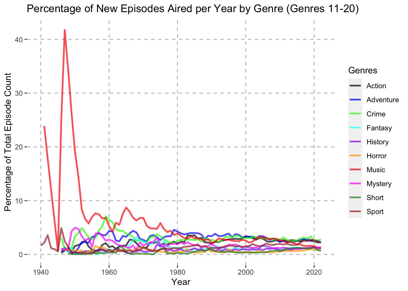
genre_split %>%
group_by(genres, startYear) %>%
summarise(numberOfEpisodes = n()) %>%
filter(genres %in% twenty_one_to_twenty_eight_genres$genres) %>%
ggplot(aes(x = startYear, y = numberOfEpisodes, color = genres)) +
geom_line(linewidth = 1, alpha = 0.7) +
scale_color_manual(values = color_palette) +
labs(x = "Year", y = "Number of Episodes", color = "Genres") +
ggtitle("Number of New Episodes Aired per Year by Genre (Genres 21-28)") +
theme(panel.background = element_rect(fill = "white")) +
theme(panel.grid.major = element_line(color = "gray", linetype = "dashed"))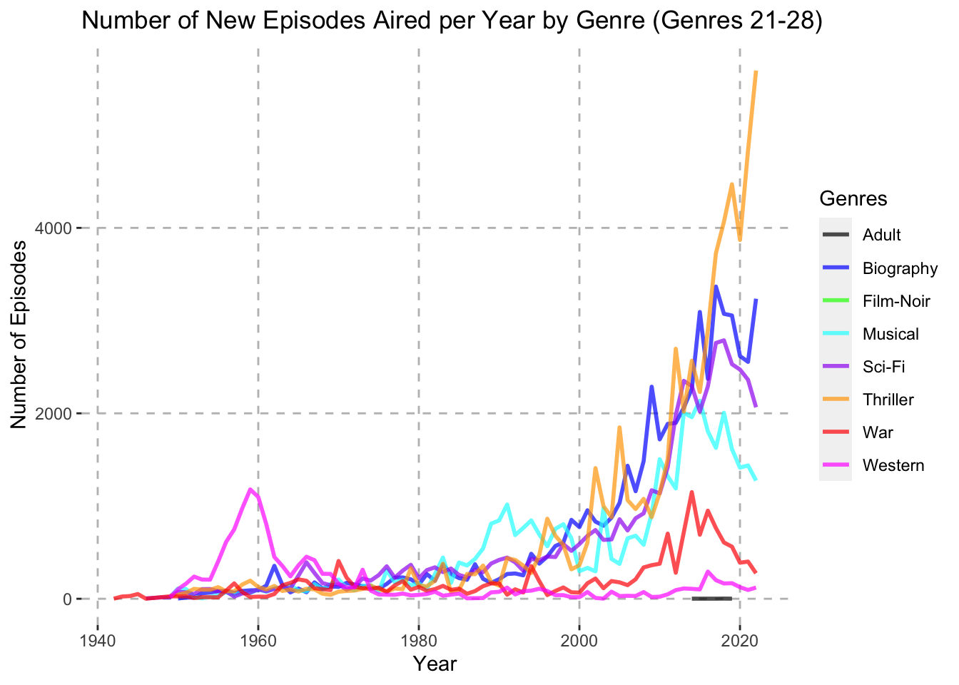
genre_split %>%
group_by(genres, startYear) %>%
summarise(numberOfEpisodes = n()) %>%
group_by(startYear) %>%
mutate(percentage = numberOfEpisodes / sum(numberOfEpisodes) * 100) %>%
filter(genres %in% twenty_one_to_twenty_eight_genres$genres) %>%
ggplot(aes(x = startYear, y = percentage, color = genres)) +
geom_line(linewidth = 1, alpha = 0.7) +
scale_color_manual(values = color_palette) +
labs(x = "Year", y = "Percentage of Total Episode Count", color = "Genres") +
ggtitle("Percentage of New Episodes Aired per Year by Genre (Genres 21-28)") +
theme(panel.background = element_rect(fill = "white")) +
theme(panel.grid.major = element_line(color = "gray", linetype = "dashed"))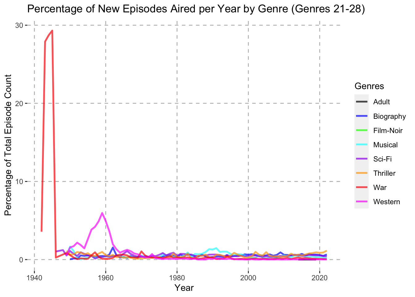
One interesting take away from the Percentage of New Episodes Aired per Year by Genre (Genres 11-20) plot is that around 1947 over 40% of all new episodes aired fell under the Music category. During this time of course there were very few TV series episodes released in general, but this is still an interesting finding. Also, another interesting trend can be seen from the Number of New Episodes Aired per Year by Genre (Genres 21-29) chart. Here we can see that the Western genre spiked during the late fifties and early sixties to around 5% of all new episodes aired. It then fell and remained quite low for the rest of the time period.
One limitation of these plots is that they only look at the number of episodes released per year for each genre. It could be beneficial to also examine how the viewer ratings of specific genres change over time. This could reveal if there are correlations between a specific genre becoming more popular and viewers giving episodes of that genre a higher rating. Since we have identified trends in the Talk-Show, News, Reality-TV, Music, and Western genres in terms of their percentage share of new episodes aired, we can look at how the average rating of these genres changed over time and compare the trends.
genres_of_interest <- c("Talk-Show", "News", "Reality-TV", "Music", "Western")
color_palette <- c("black", "blue", "green", "red", "purple")
genre_split %>%
group_by(genres, startYear) %>%
summarise(averageRating = mean(averageRating, na.rm = TRUE)) %>%
filter(genres %in% genres_of_interest) %>%
ggplot(aes(x = startYear, y = averageRating, color = genres)) +
geom_line(linewidth = 1, alpha = 0.7) +
scale_color_manual(values = color_palette) +
labs(x = "Year", y = "Average Viewer Rating", color = "Genres") +
ggtitle("Average Viewer Rating per Year by Genre") +
theme(panel.background = element_rect(fill = "white")) +
theme(panel.grid.major = element_line(color = "gray", linetype = "dashed"))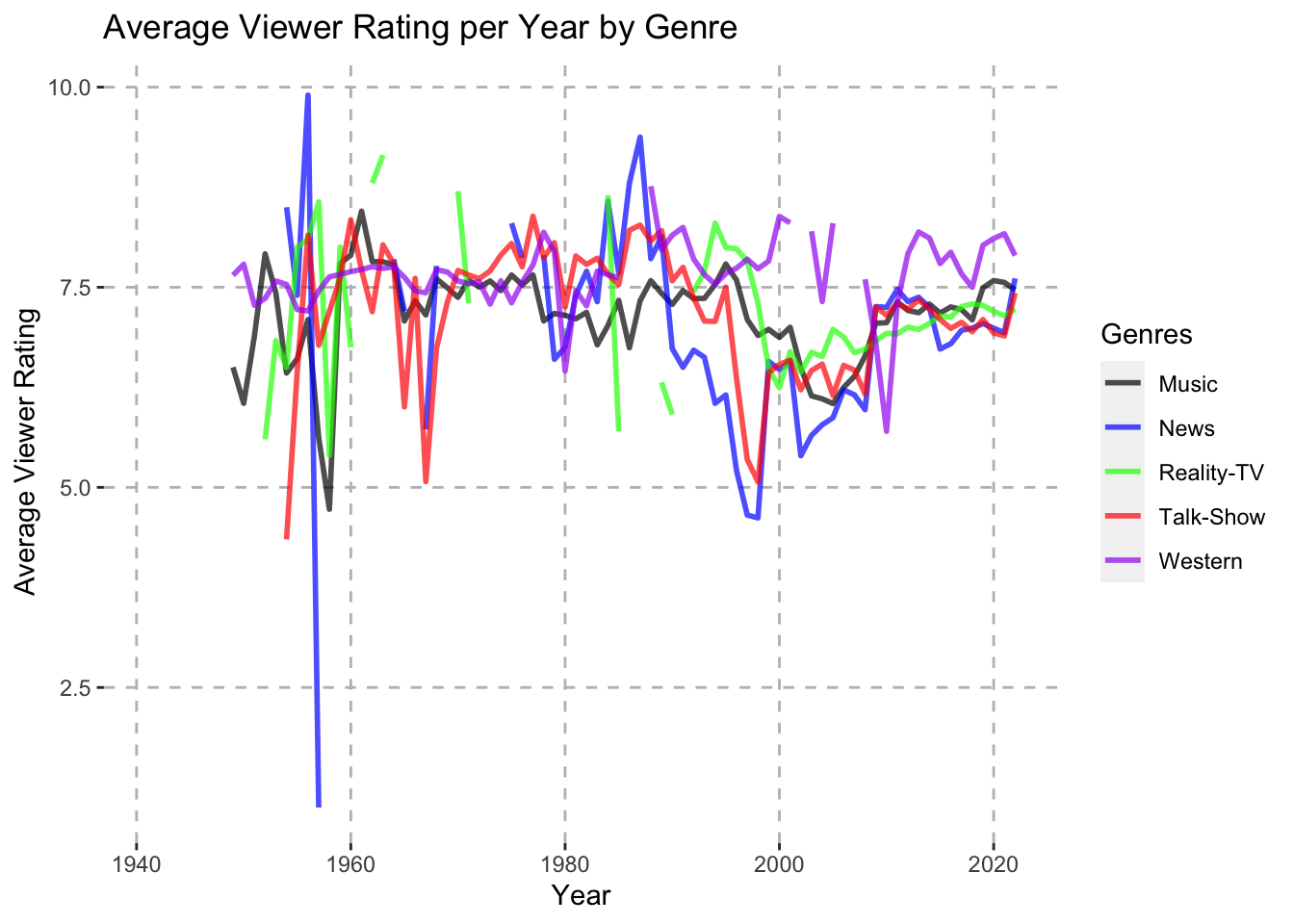
From the Average Viewer Rating per Year by Genre graph, we can see that the Talk-Show, News, and Reality-TV genres did increase in terms of average viewer rating during the 2000’s, which aligns with their trend from the Percentage of New Episodes Aired per Year by Genre (Top 10 Genres) graph. However, this time was not when their average viewer ratings were the highest, which occurred at various points between the 60’s and 90’s. Also, despite the Western genre taking up a much higher percentage of the total episodes aired during the 60’s, its average viewer rating was actually highest between the 90’s and 2020. Finally, although the Music genre made up over 40% of all new episodes aired around 1947, it did not have a spike in its average viewer rating during this time. In comparing this plot to the Percentage of New Episodes Aired per Year by Genre graphs, it appears that more episodes of a genre being produced does not necessarily correlate to an increased average viewer score.
In order to examine the trend between the length of a series and its popularity, we first need to group episodes by their parent series so that we can count the number of episodes in each series. We can also average the viewer ratings for each episode to get an overall series rating. For this analysis we will use the episodes_rated data frame since we want to only look at series which have all of their episodes rated (so that we can get an accurate series rating). Also, we will exclude series that have less than 3 episodes.
series <- episodes_rated %>%
select(seriesID, startYear, averageRating) %>%
group_by(seriesID) %>%
summarise(numberEpisodes = n(), seriesRating = mean(averageRating)) %>%
filter(numberEpisodes >= 3)
seriesggplot(series, aes(x = numberEpisodes, y = seriesRating)) +
geom_point(alpha = 0.3, color = "blue") +
labs(x = "Number of Episodes", y = "Average Series Viewer Rating") +
ggtitle("Number of Episodes vs. Average Series Viewer Rating (At Least 3 Episodes)") +
theme(panel.background = element_rect(fill = "white")) +
theme(panel.grid.major = element_line(color = "gray", linetype = "dashed"))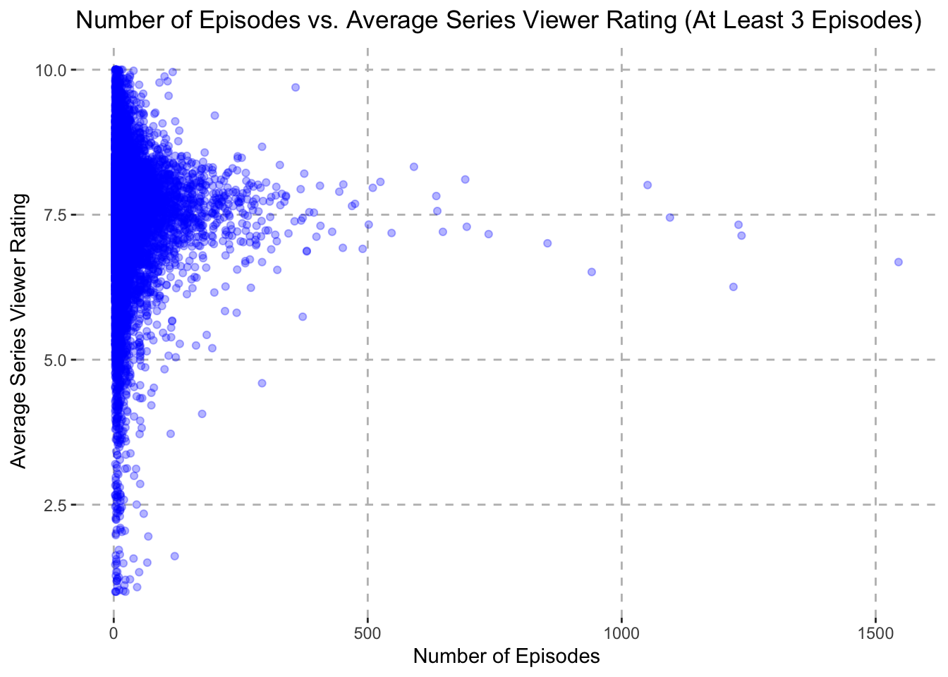
From the plot we can see that the vast majority of series in the data set have less than 250 episodes and their ratings are widely distributed. Still, the most common rating for these series is around 7.5. What is more interesting is that nearly all series that have more than 250 episodes are rated at at least 6.25, with an average of around 7.5. This may be indicative that to have a series continue to produce new episodes, it is necessary for viewers to like the series.
From the analysis and visualizations generated in this project, we were able to examine several trends within the TV series data supplied by IMDb. We were able to discover that the average viewer rating of all TV series episodes has remained fairly constant across the history of TV episodes, however the number of episodes released each year grew steadily and then skyrocketed during the 2000’s. Also, we noted that the average number of viewer ratings for episodes aired prior to the creation of IMDb was in general much lower than that of episodes released once IMDb came into existence. This may hint that users of the platform are more motivated to rate an episode around its release date when they view it for the first time. One limitation of the data set that may be an interesting factor to explore in the future is weighing the audience population against these trends. The global population increased significantly since the starting point of the data (around 1940), as did access to televisions and other viewing devices. These are definitely large factors that would have increased demand for new shows.
Furthermore, we identified some interesting patterns for several individual genres, both in terms of total episodes aired and percentage of total episodes aired. In looking at the average viewer ratings for these genres over time, we saw that an increase in a genres’ percentage of all episodes aired during a year does not necessarily correlate to an increased average viewer score for that genre during that year. One limitation of this data set in terms of studying individual genres is that it does not give information about the individual users of IMDb. It is possible that the type of people who actively rate episodes on IMDb tend to prefer certain genres over others, thereby rating them higher or more often. Therefore, it may be interesting to examine user rating tendencies in terms of genre among IMDb users in order to explain trends for specific genres.
Finally, by comparing the number of series episodes to average viewer rating of all episodes in the series, we noted that all extensive series’ (over 250 episodes) were rated at least 6.25. This likely indicates that for a series to continue to be funded over a long period of time, it needs to be viewed positively by its audience so that they will continue to watch new episodes. One limitation of the data set here is that we do not have access to information about the budget for TV series seasons or episodes. With this information, we could take a closer look at how the budget for subsequent seasons or episodes changed as a series became older. This might help identify a trend between average viewer rating and budget over time.
“IMDb Non-Commercial Datasets.” IMDb Developer, 13 June 2023, datasets.imdbws.com/.
Khetlani, Komal. “IMDb Dataset - from 1888 to 2023.” Kaggle, 5 Apr. 2021, www.kaggle.com/datasets/komalkhetlani/imdb-dataset.
Lewis, Robert. “IMDb.” Encyclopedia Britannica, 15 May 2023, www.britannica.com/topic/IMDb.
R Core Team (2023). R: A Language and Environment for Statistical Computing. R Foundation for Statistical Computing, Vienna, Austria. https://www.R-project.org/.
“Ratings FAQ.” IMDb, 9 May 2023, help.imdb.com/article/imdb/track-movies-tv/ratings-faq/G67Y87TFYYP6TWAV#.
“Where Does the Information on IMDb Come From?” IMDb, 9 May 2023, help.imdb.com/article/imdb/general-information/where-does-the-information-on-imdb-come-from/GGD7NGF5X3ECFKNN.
Wickham, Hadley, et al. R for Data Science: Import, Tidy, Transform, Visualize, and Model Data. 2nd ed., O’Reilly Media, Inc, 2023.