Code
library(tidyverse)
library(readxl)
library(lubridate)
knitr::opts_chunk$set(echo = TRUE, warning=FALSE, message=FALSE)library(tidyverse)
library(readxl)
library(lubridate)
knitr::opts_chunk$set(echo = TRUE, warning=FALSE, message=FALSE)For the final project I have chosen to use a data set containing information about TV series listed on IMDb (Internet Movie Database) to examine viewer opinions of TV series quality. The data I will be using are comprised of three files. The title.basics.tsv file contains data about all the titles on IMDb including movies, TV series, individual TV episodes, shorts, etc. The title.episode.tsv file maps TV episode titles to their parent TV series title, and also includes the season and episode number. The title.ratings.tsv file contains the rating for each title.
Let’s read in the title.basics.tsv data and examine the rows
title_basics <- read_tsv("noah_data/title.basics.tsv")
title_basicsAs we can see the data frame is very large (over 9 million rows). However, the data we will actually use for analysis will be much less after cleaning. Each row in the data frame represents one “title” (could be a movie, TV series, individual TV episode, short, etc.). A description of each of the data columns is as follows:
- tconst: alphanumeric unique identifier of the title
- titleType: the type/format of the title (e.g. movie, short, TV series, TV episode, video, etc.)
- primaryTitle: the more popular title / the title used by the filmmakers on promotional materials at the point of release
- originalTitle: original title, in the original language
- isAdult: 0: non-adult title; 1: adult title
- startYear: represents the release year of a title. In the case of TV Series, it is the series start year
- endYear: TV Series end year. ‘’ for all other title types
- runtimeMinutes: primary runtime of the title, in minutes
- genres: includes up to three genres associated with the title
The code below reveals the data types of the data columns.
spec(title_basics)cols(
tconst = col_character(),
titleType = col_character(),
primaryTitle = col_character(),
originalTitle = col_character(),
isAdult = col_double(),
startYear = col_character(),
endYear = col_character(),
runtimeMinutes = col_character(),
genres = col_character()
)Similarly, lets read in and describe the title.episode.tsv file.
title_episode <- read_tsv("noah_data/title.episode.tsv")
title_episodeA description of each of the data columns in this data frame is as follows:
- tconst: alphanumeric identifier of episode
- parentTconst: alphanumeric identifier of the parent TV Series
- seasonNumber: season number the episode belongs to
- episodeNumber: episode number of the tconst in the TV series
The code below reveals the data types of the data columns.
spec(title_episode)cols(
tconst = col_character(),
parentTconst = col_character(),
seasonNumber = col_character(),
episodeNumber = col_character()
)Finally, lets read in and describe the title.ratings.tsv file.
title_ratings <- read_tsv("noah_data/title.ratings.tsv")
title_ratingsA description of each of the data columns in this data frame is as follows:
- tconst: alphanumeric identifier of episode
- averageRating: weighted average of all the individual user ratings
- numVotes: number of rating votes the title has received
The code below reveals the data types of the data columns.
spec(title_ratings)cols(
tconst = col_character(),
averageRating = col_double(),
numVotes = col_double()
)The goal of the data tidying will be to consolidate the information from the three data files into two data frames that can be used for analysis. Each case in the data frames should represent an episode of a TV series. The data frames will have columns that include the episodes average viewer rating, number of rated votes, the name and identifier of the series the episode belongs to, and the season and episode numbers. The difference between the two data frames will be that one will contain all TV series episodes in the data set, and the other will only contain episodes that belong to series which have all episodes rated by viewers (no NA values).
First, we will drop all non TV Episodes from the title_basics data frame to get a data frame of all titles that are TV episodes. We will also remove adult TV episodes.
episodes_all <- subset(title_basics, titleType == "tvEpisode" & isAdult == 0)
episodes_allNow, we will perform a left outer join between the episodes data frame and the title_ratings data frame, to add the rating and the number of votes to the episodes data frame.
episodes_all <- left_join(episodes_all, title_ratings, by = "tconst")
episodes_allNow, we will perform another left outer join between the episodes data frame and the title_episode data frame, to add the parent TV series identifier, the season number, and episode number to the episode data frame.
episodes_all <- left_join(episodes_all, title_episode, by = "tconst")
episodes_allNow, lets add the series title to each episode case.
episodes_all <- episodes_all %>%
left_join(title_basics %>% select(tconst, primaryTitle), by = c("parentTconst" = "tconst"))
episodes_allLets now clean up the data by renaming columns and removing columns we don’t need. In particular we will remove the titleType column since it is always “tvEpisode”, the originalTitle column since the primaryTitle column is sufficient, the isAdult column since it is always 0, and the endYear column since we are not concerned with when a show ended. We will use the number of episodes, seasons, and run times to compare shows by length.
episodes_all <- select(episodes_all, seriesID = parentTconst, seriesName = primaryTitle.y, episodeID = tconst, episodeName = primaryTitle.x, startYear, runtimeMinutes, genres, averageRating, numVotes, seasonNumber, episodeNumber)
episodes_allFinally, lets change the numerical columns to integers rather than chars, change the startYear column to a date format, and remove dates outside the range 1940-2022.
episodes_all <- mutate(episodes_all, startYear = as.Date(paste0(startYear, "-01-01"), format = "%Y-%m-%d"), runtimeMinutes = as.integer(runtimeMinutes), seasonNumber = as.integer(seasonNumber), episodeNumber = as.integer(episodeNumber)) %>%
filter(startYear < as.Date("2023-01-01") & startYear > as.Date("1939-01-01"))
episodes_allThe data frame is now tidied, with each case representing an episode of a TV series. However, not all of the TV series episodes have an average rating (several rows have NA for this column). It will be helpful in our analysis to have access to a data frame that contains only the episodes that belong to series for which all episodes have a rating. In order to make this data frame, first we need to make a set of all the series identifiers (seriesID) that have at least one episode with no ratings.
unrated_series <- unique(episodes_all$seriesID[is.na(episodes_all$averageRating)])
length(unrated_series)[1] 159049There are 159,049 series with at least one episode that is unrated. Now, we will remove all episodes of these series and store the result in a new data frame.
episodes_rated <- subset(episodes_all, !(seriesID %in% unrated_series))
episodes_ratedWe now have two tidied data frames for analysis. The episodes_all data frame contains all TV series episodes, while the episodes_rated data frame contains all of the TV series episodes that have a rating and belong to a TV series with each episode rated. Each column in both data frames is labeled appropriately with a descriptive name and the data types make sense for this data set. A final description of the data in each column of the two data frames is:
- seriesID: a unique identifier for the TV series
- seriesName: the name of the series
- episodeID: a unique identifier for the series episode
- episodeName: the name of the episode
- startYear: the year the series started
- runtimeMinutesv: the runtime of the series in minutes
- averageRating: the average viewer rating of the episode
- numVotes: the number of rating votes the episode received
- seasonNumber: the number of the season
- episodeNumber: the number of the episode
A few research questions that will be answered with this data set are:
1. How have TV series improved over time in terms of quality and quantity?
2. What do popularity and frequency trends of certain genres of TV shows look like over time?
3. Does a longer TV series indicate a higher quality series?
In order to examine how TV series episode quality and quantity has evolved over time, we can group TV series episodes by their startYear (year when the episode aired). We can then compute statistics on these groups such as the average rating of all episodes that aired this year, as well as the count of the number of episodes that aired this year.
quantity_quality <- episodes_all %>%
select(startYear, averageRating) %>%
group_by(startYear) %>%
summarise(averageRating = mean(averageRating, na.rm = TRUE), totalEpisodes = n())
quantity_qualityFrom the output we can see that the average viewer rating of all TV series episodes has remained fairly constant from 1948-2023 at around 7.0-7.5. However, it is evident that the number of TV series episodes produced per year has increased each year. We can plot these results to better understand the trends of quantity and quality of TV series episodes over time.
ggplot(quantity_quality, aes(x = startYear, y = averageRating)) +
geom_line(color = "red") +
theme_minimal() +
labs(title = "Average Viewer Rating vs Time", x = "Year", y = "Average Viewer Rating") +
ylim(0, 10)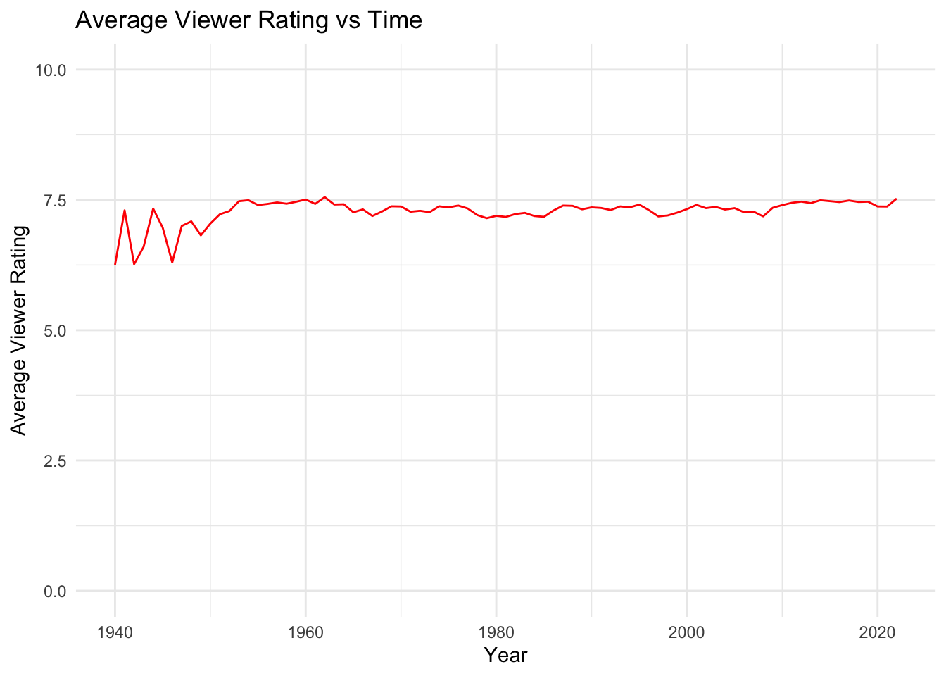
ggplot(quantity_quality, aes(x = startYear, y = totalEpisodes)) +
geom_line(color = "blue") +
theme_minimal() +
labs(title = "Number of New Episodes Aired vs Time", x = "Year", y = "Number of Episodes")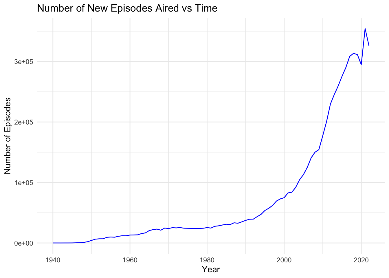
From the Average Viewer Rating vs Time graph above we can confirm our previous observation that the average TV series episodes rating has remained fairly constant from 1940-2022. There appears to be some larger variations among the years between 1940 and 1950, however this is likely due to the fact that the sample size is much smaller (less TV episodes were released this year). This can be seen in the second graph, the Number of New Episodes Aired vs Time. In this graph it is evident that between 1940 and 2020, the number of TV series episodes has grown exponentially. We can see that the rate at which the number of episodes produced jumped drastically during the mid 2000’s. This could be due to the explosion of streaming services during this time, allowing viewers to consume series more quickly by binging them. It is also interesting to note that the amount of new episodes aired dropped in 2020, which could be due to the COVID-19 pandemic. Episode production likely slowed down during this time which may have resulted in several seasons or individual episodes moving back their release dates.
One limitation of these visualizations is that they only look at the average viewer rating of all TV series over time. However, since the number of epsiodes released has changed drastically over the time period of the data set, it might be beneficial to also look at other statistics such as the median, mode, and standard deviation of viewer ratings for specific years or buckets of years. This might help draw better conclusions about how viewer ratings have changed over time.
In order to examine the popularity trends of genres over time, we will first split the rows so that each row only contains one genre (episodes with more than one genre will have more than one row, each representing one genre).
genre_split <- episodes_all %>%
separate_rows(genres, sep = ",")
genre_splitNow that each row only has one genre, we can group by genre to see ho w many genres the data set contains.
genre_count <- genre_split %>%
group_by(genres) %>%
summarise(numberOfEpisodes = n()) %>%
arrange(desc(numberOfEpisodes))
genre_countSince 29 genres is too many to plot at once, we will start by looking at the top 10 most common genres to see how they have evolved over time.
top_ten_genres <- genre_count %>%
head(10)genre_split %>%
group_by(genres, startYear) %>%
summarise(numberOfEpisodes = n()) %>%
filter(genres %in% top_ten_genres$genres) %>%
ggplot(aes(x = startYear, y = numberOfEpisodes, color = genres)) +
geom_line() +
labs(x = "Year", y = "Number of Episodes", color = "Genres") +
ggtitle("Number of New Episodes Aired per Year by Genre (Top Ten Genres)")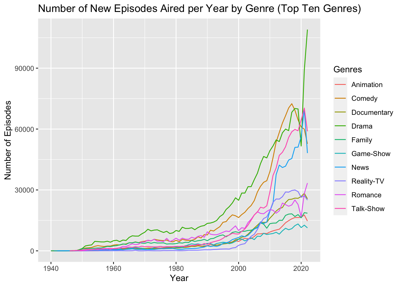
We can see from the Number of New Episodes Aired per Year by Genre graph that several genres grew substantially in terms of episode releases during the mid 2000’s, namely Drama, Comedy, Talk-Show, and News. While it is clear these genres had a sharp increase in the number of new episodes aired, it is difficult to discern whether or not these genres actually became more popular in terms of the total percentage of new shows created. Their growth during the mid 2000’s could just come as a result of more shows being produced overall, and therefore it might be beneficial to look at the percentage of total shows released in each year that fall under each of these genres instead.
genre_split %>%
group_by(genres, startYear) %>%
summarise(numberOfEpisodes = n()) %>%
group_by(startYear) %>%
mutate(percentage = numberOfEpisodes / sum(numberOfEpisodes) * 100) %>%
filter(genres %in% top_ten_genres$genres) %>%
ggplot(aes(x = startYear, y = percentage, color = genres)) +
geom_line() +
labs(x = "Year", y = "Percentage of Total Count", color = "Genres") +
ggtitle("Percentage of New Episodes Aired per Year by Genre (Top Ten Genres)")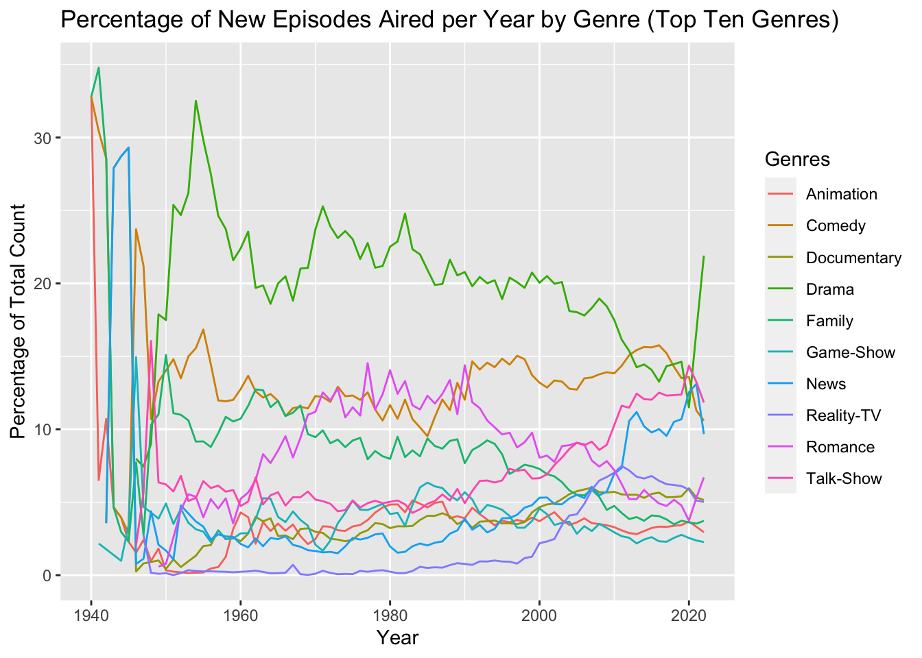
From the Percentage of New Episodes Aired per Year by Genre (Top Ten Genres) graph, we can see that Talk-Show and News genres did indeed increase during the 2000’s in terms of percentage of total new episodes aired. However, the Drama genre did not increase during the early and mid 2000’s, though it skyrocketed from 2020-2022. The Comedy genre mostly remained constant throughout the 2000’s. One of the more notable trends in this graph is Reality-TV, which made up almost none of the new episodes released until 2000. It then rose over the 2000’s to eventually make up nearly 8% of all new episode releases.
Let’s now look at the other 19 genres.
ten_to_twenty_genres <- genre_count %>%
slice(11:20)
twenty_to_thirty_genres <- genre_count %>%
slice(21:29)
genre_split %>%
group_by(genres, startYear) %>%
summarise(numberOfEpisodes = n()) %>%
filter(genres %in% ten_to_twenty_genres$genres) %>%
ggplot(aes(x = startYear, y = numberOfEpisodes, color = genres)) +
geom_line() +
labs(x = "Year", y = "Number of Episodes", color = "Genres") +
ggtitle("Number of New Episodes Aired per Year by Genre (Genres 11-20)")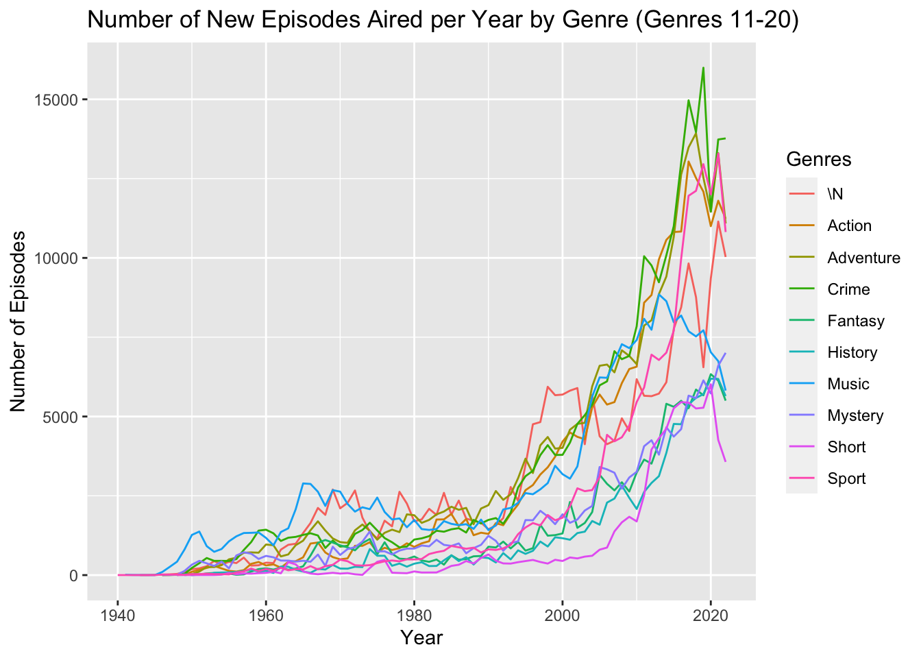
genre_split %>%
group_by(genres, startYear) %>%
summarise(numberOfEpisodes = n()) %>%
group_by(startYear) %>%
mutate(percentage = numberOfEpisodes / sum(numberOfEpisodes) * 100) %>%
filter(genres %in% ten_to_twenty_genres$genres) %>%
ggplot(aes(x = startYear, y = percentage, color = genres)) +
geom_line() +
labs(x = "Year", y = "Percentage of Total Count", color = "Genres") +
ggtitle("Percentage of New Episodes Aired per Year by Genre (Genres 11-20)")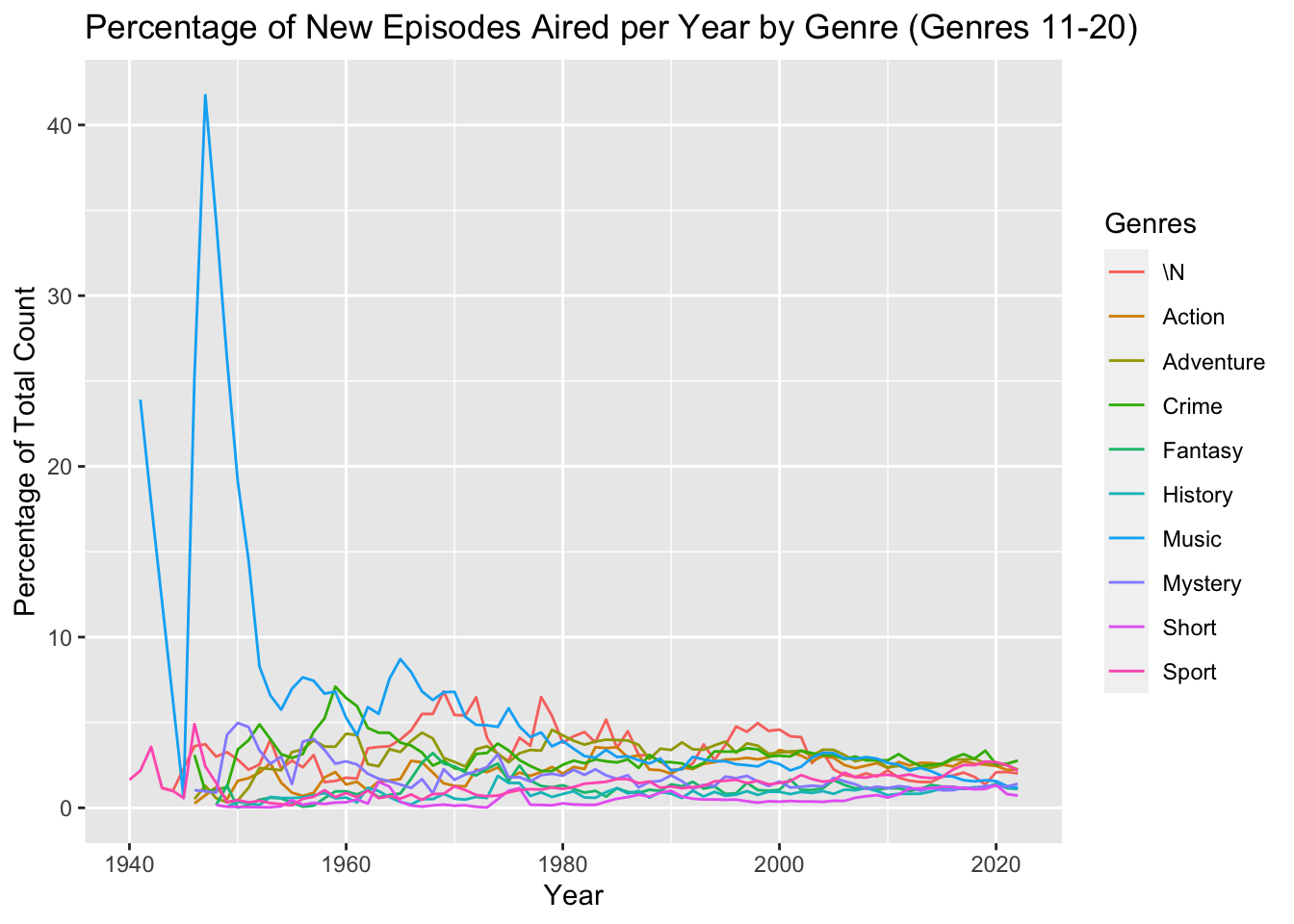
genre_split %>%
group_by(genres, startYear) %>%
summarise(numberOfEpisodes = n()) %>%
filter(genres %in% twenty_to_thirty_genres$genres) %>%
ggplot(aes(x = startYear, y = numberOfEpisodes, color = genres)) +
geom_line() +
labs(x = "Year", y = "Number of Episodes", color = "Genres") +
ggtitle("Number of New Episodes Aired per Year by Genre (Genres 21-29)")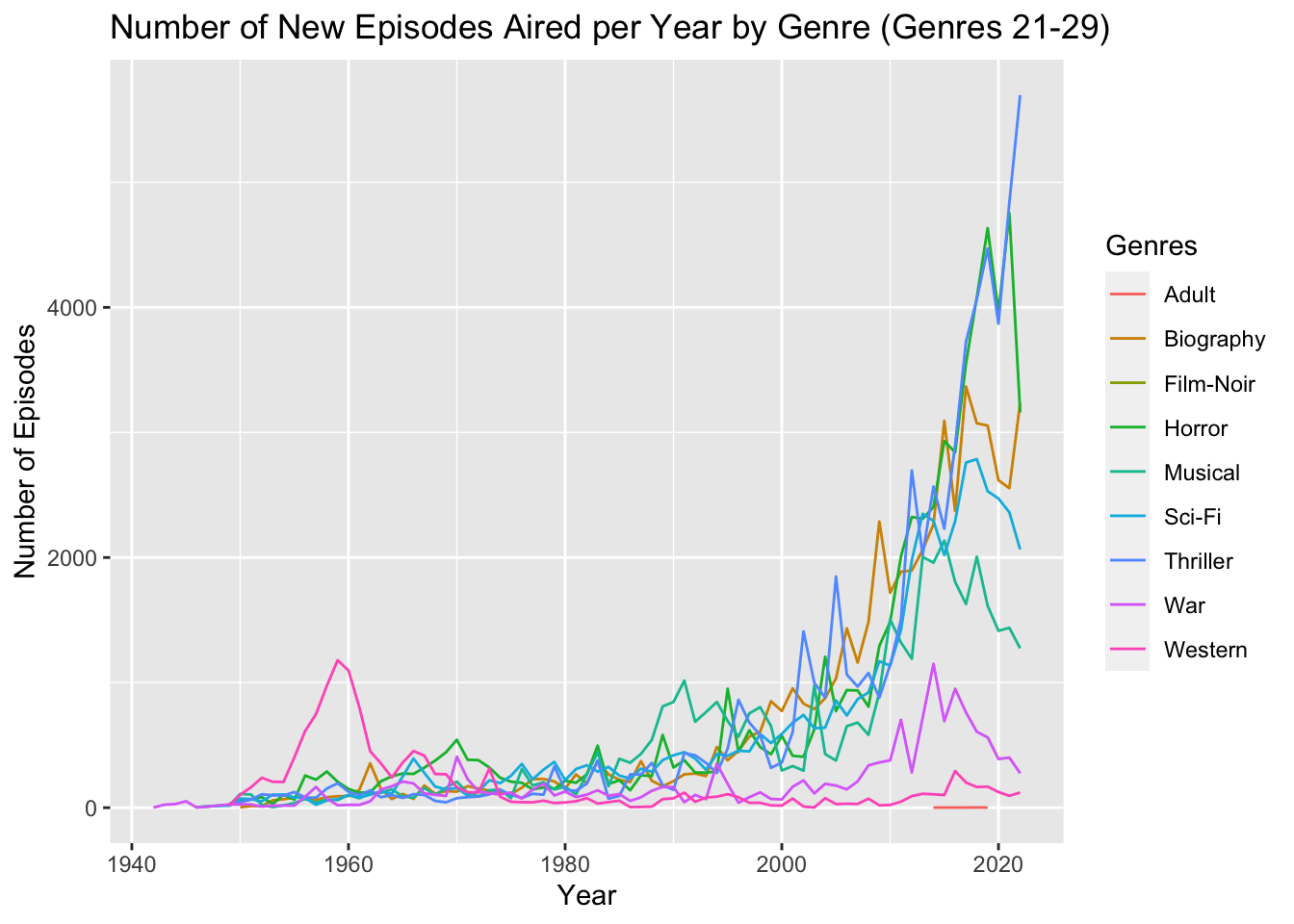
genre_split %>%
group_by(genres, startYear) %>%
summarise(numberOfEpisodes = n()) %>%
group_by(startYear) %>%
mutate(percentage = numberOfEpisodes / sum(numberOfEpisodes) * 100) %>%
filter(genres %in% twenty_to_thirty_genres$genres) %>%
ggplot(aes(x = startYear, y = percentage, color = genres)) +
geom_line() +
labs(x = "Year", y = "Percentage of Total Count", color = "Genres") +
ggtitle("Percentage of New Episodes Aired per Year by Genre (Genres 21-29)")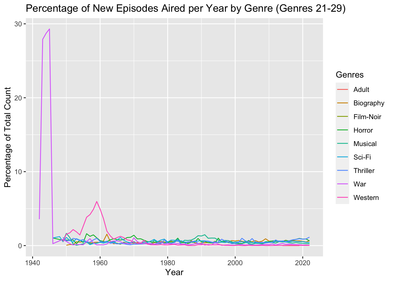
One interesting trend we can see from the Number of New Episodes Aired per Year by Genre (Genres 21-29) is that the Western genre spiked heavily during the late fifties and early sixties.
One limitation of these plots is that they only look at the number of epsiodes released per year for each genre. It could be beneficial to also examine how the viewer ratings of specific genres change over time. This could reveal when the best series of a specific genre were released rather than just the quantity of series of a specific genre.
In order to examine the trend between the length of a series and it’s popularity, we first need to group episodes by their parent series so that we can count the number of episodes in each series. We can also average the viewer ratings for each episode to get an overall series rating. For this analysis we will use the episodes_rated data frame since we want to only look at series which have all of their episodes rated (so that we can get an accurate series rating). Also, we will exclude series that have less than 3 episodes.
series <- episodes_rated %>%
select(seriesID, startYear, averageRating) %>%
group_by(seriesID) %>%
summarise(numberEpisodes = n(), seriesRating = mean(averageRating)) %>%
filter(numberEpisodes >= 3)
seriesggplot(series, aes(x = numberEpisodes, y = seriesRating)) +
geom_point() +
labs(x = "Number of Episodes", y = "Series Rating") +
ggtitle("Number of Episodes vs. Series Rating (At Least 3 Episodes)") 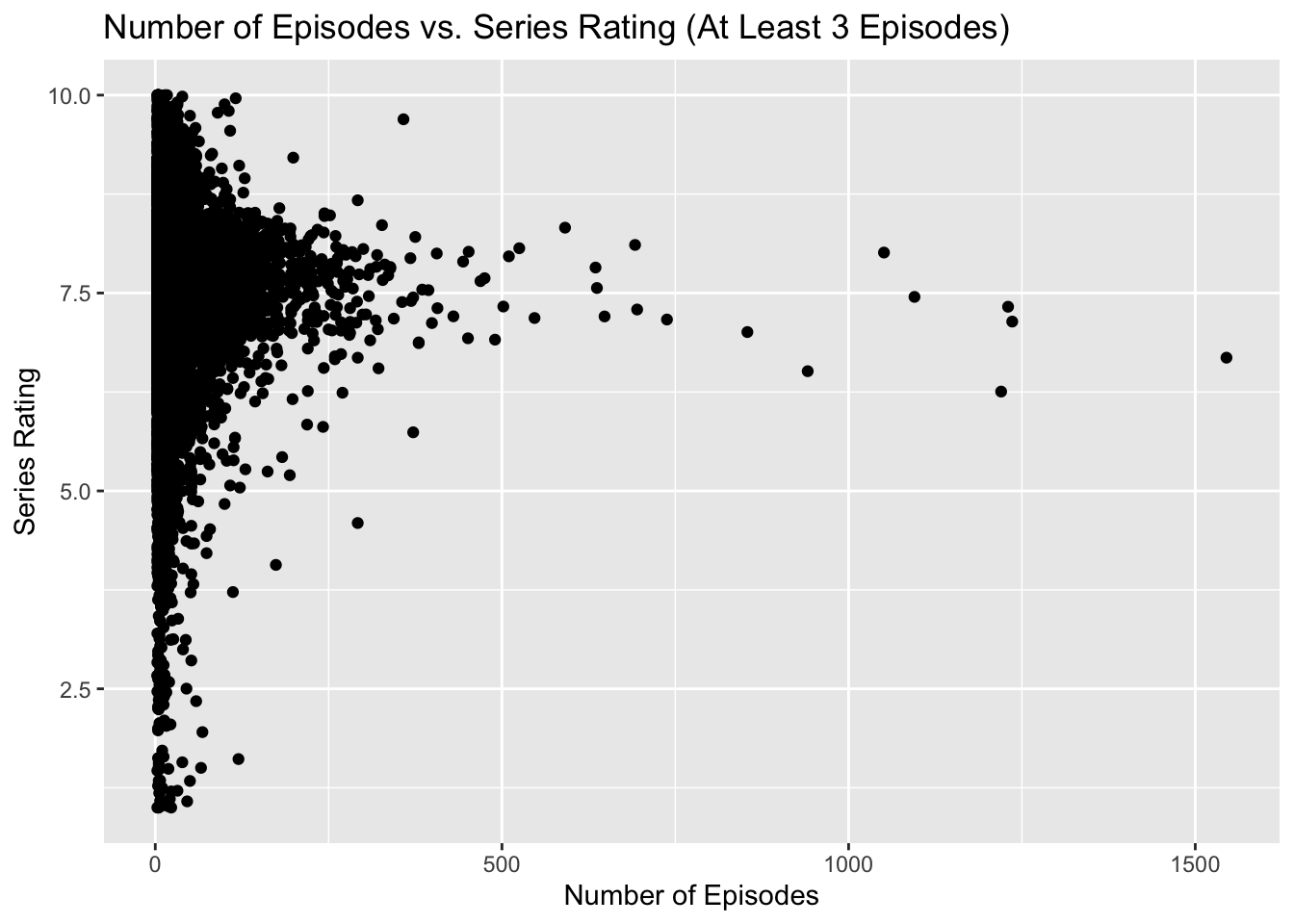
From the plot we can see that the vast majority of series in the data set have less than 250 episodes and their ratings are widely distributed. Still, the most common rating for these series is around 7.5. What is more interesting is that nearly all series that have more that 250 episodes are rated at at least 6.25, with an average of arounnd 7.5. This is indiciative of the fact that to have a series continue to produce new episodes, it is usually a requirement that viewers like the series.
One limitation of this visualization is that it does not include numerical descriptive statistics of the series rating distribution or number of episodes distribution. In drawing conclusions about how series viewer ratings relate to the length of a series it may be helpful to have concrete descriptive statistical values. Also, this visualization only uses the number of episodes to describe the length of a series, but does not take into account the episode runtimes or the number of seasons. These may be interesting dimensions to introuce into this section to further examine series length vs series rating.