Final Project - Olympics

Analysis on Olympics from 1896 to 2016

Code

library(tidyverse)
library(ggplot2)
library(treemap)

knitr::opts_chunk$set(echo = TRUE, warning=FALSE, message=FALSE)

Overview

For my final project, I would do exploratory analysis on the Olympics data right from the year it started in 1896 in Athena till 2016 in Rio de Janeiro.

Olympics

Olympics is the most decorated sporting event in an athlete’s career. The Olympics are the leading international sporting events featuring summer and winter sports competitions in which thousands of athletes from around the world participate in a variety of competitions. The Olympic Games are considered the world’s foremost sports competition with more than 200 teams, representing sovereign states and territories, participating. The Olympic Games are normally held every four years, and since 1994, have alternated between the Summer and Winter Olympics every two years during the four-year period. The first, second, and third place finishers in each event receive Olympic medals: gold, silver, and bronze, respectively.

Dataset

The dataset I would use for this analysis is downloaded from Kaggle. The original data has been scraped from https://www.sports-reference.com/ in May 2018 and cleaned by Samruddhi Mhatre.

This dataset consists of Olympics data of over a century, from the year 1896 to 2016. Studying this dataset will help to understand the patterns followed in the games of Olympics, patterns of the most successful athletes and countries in their Olympics journey and much more!

Code

olympics_data <- read_csv("_data/athlete_events_olympics.csv")
olympics_data

The data set has 271116 observations and 15 data points recorded per observation. Each observation records variables like ID, Name, Sex, Age, Height, Weight, Team, NOC, Games, Year, Season, City, Sport, Event, Medal.

The youngest and the oldest athlete that ever participated are 10 and 97 years of age respectively. Athletes from across the world compete in 765 events that happen across 66 sports. These happen in 2 Olympic seasons i.e Summer, Winter.

Data Cleaning

The dataset is mostly clean and we don’t have to work around much. Although, for doing some analysis, we might need to create various subsets of data like medals, teams, etc, drop na values for a few variables and mutate new variables(Most of these can be done during the analysis). We need to convert categorical variables into factor to get overall summary across various variables. We don’t need the “ID” column for our analysis as it only serves the purpose of a key.

Code

olympics_data <- olympics_data %>%
  mutate_if(is_character, as.factor) %>%
  select(-ID)

medals <- olympics_data %>%
  filter(!is.na(Medal))

summary(olympics_data)

                       Name        Sex             Age            Height     
 Robert Tait McKenzie    :    58   F: 74522   Min.   :10.00   Min.   :127.0  
 Heikki Ilmari Savolainen:    39   M:196594   1st Qu.:21.00   1st Qu.:168.0  
 Joseph "Josy" Stoffel   :    38              Median :24.00   Median :175.0  
 Ioannis Theofilakis     :    36              Mean   :25.56   Mean   :175.3  
 Takashi Ono             :    33              3rd Qu.:28.00   3rd Qu.:183.0  
 Alexandros Theofilakis  :    32              Max.   :97.00   Max.   :226.0  
 (Other)                 :270880              NA's   :9474    NA's   :60171  
     Weight                 Team             NOC                 Games       
 Min.   : 25.0   United States: 17847   USA    : 18853   2000 Summer: 13821  
 1st Qu.: 60.0   France       : 11988   FRA    : 12758   1996 Summer: 13780  
 Median : 70.0   Great Britain: 11404   GBR    : 12256   2016 Summer: 13688  
 Mean   : 70.7   Italy        : 10260   ITA    : 10715   2008 Summer: 13602  
 3rd Qu.: 79.0   Germany      :  9326   GER    :  9830   2004 Summer: 13443  
 Max.   :214.0   Canada       :  9279   CAN    :  9733   1992 Summer: 12977  
 NA's   :62875   (Other)      :201012   (Other):196971   (Other)    :189805  
      Year         Season                   City               Sport       
 Min.   :1896   Summer:222552   London        : 22426   Athletics : 38624  
 1st Qu.:1960   Winter: 48564   Athina        : 15556   Gymnastics: 26707  
 Median :1988                   Sydney        : 13821   Swimming  : 23195  
 Mean   :1978                   Atlanta       : 13780   Shooting  : 11448  
 3rd Qu.:2002                   Rio de Janeiro: 13688   Cycling   : 10859  
 Max.   :2016                   Beijing       : 13602   Fencing   : 10735  
                                (Other)       :178243   (Other)   :149548  
                                 Event           Medal       
 Football Men's Football            :  5733   Bronze: 13295  
 Ice Hockey Men's Ice Hockey        :  4762   Gold  : 13372  
 Hockey Men's Hockey                :  3958   Silver: 13116  
 Water Polo Men's Water Polo        :  3358   NA's  :231333  
 Basketball Men's Basketball        :  3280                  
 Cycling Men's Road Race, Individual:  2947                  
 (Other)                            :247078                  

Code

olympics_data

Code

medals

Insights

Code

#Type of medals won by teams.
teams_medals_type <- medals %>%
  group_by(NOC, Medal) %>%
  summarise(count = n())

#Total medals won by teams
teams_medals_total <- medals %>%
  group_by(NOC) %>%
  summarise(total_medals = n()) %>%
  arrange(desc(total_medals))

#Top 50 countries(by total medals won) medal_type tally.
(teams_medals_tally <- inner_join(teams_medals_type,
                              teams_medals_total[1:50, ],
                              by = "NOC") %>%
    arrange(desc(total_medals)))

Code

#Bar plot of medals won by top 50 countries.
ggplot(data = teams_medals_tally , aes(x= reorder(NOC, total_medals), y = count)) +
  geom_bar(stat = "identity",
           mapping = aes(fill = Medal),
           position = "stack") +
  scale_fill_manual(values=c('brown', 'gold', 'darkgrey')) +
  theme_classic() +
  labs(title ="Top 50 countries that won most medals",
       y = "No of medals",
       x = "Nation of Origin",
       fill = "Medal")+
  coord_flip()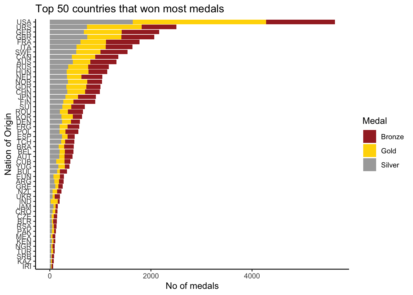

We can see that USA has won the highest number of medals, more than double the number of medals won by Soviet Union.

Code

#Sport with events count
(sport_events <- olympics_data %>%
  distinct(Sport, Event) %>%
  group_by(Sport) %>%
  summarise(no_events = n()) %>%
  arrange(desc(no_events)))

Code

#Treemap representing each Sport proportional to number of events in olympics
treemap(sport_events,
        index = "Sport",
        vSize = "no_events",
        type = "index",
        fontsize.labels = 25,
        fontcolor.labels = "black",
        align.labels=list(
          c("center", "center")),
        inflate.labels=F,
        palette = "Set1",
        title="Treemap representing each Sport proportional to number of events in olympics",
        fontsize.title=12,
        bg.labels = 0)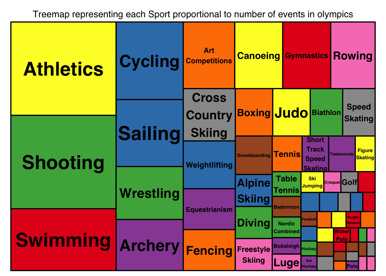

Athletics and shooting are the sports with highest number of events (83 events each) followed by swimming with 55 events.

Code

#Age distribution among females and males in olympics.
ggplot(olympics_data, aes(x = Age, na.rm = TRUE)) +
  geom_histogram(bins = 85, fill="darkred", alpha=0.7) +
  theme_linedraw() +
  facet_wrap(vars(Sex), nrow = 2, ncol = 1) +
  labs(title = "Age distribution of atheletes in Olympics",
       x = "Age",
       y = "Counts")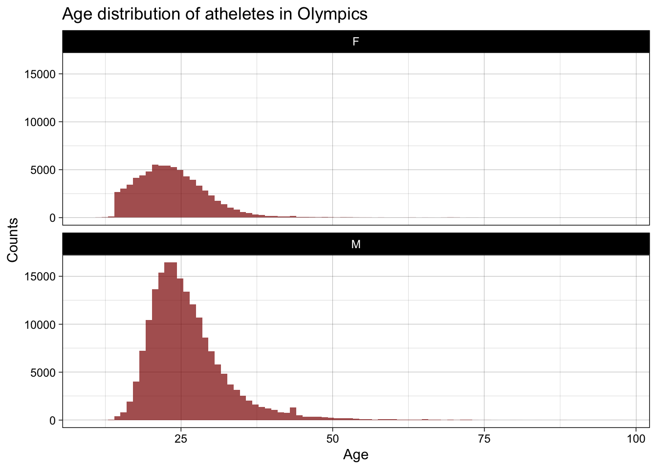

We can see that the mean age of men athletes is higher than the mean age of women athletes. Most frequent age in men athletes is approximately equal to the most frequent age in women athletes.

Code

#Times series for how top 10 nations performed over years.
teams_medals_yearly <- medals %>%
  filter(NOC %in% teams_medals_total[1:9,]$NOC) %>%
  group_by(NOC, Year) %>%
  summarise(total_medals = n()) %>%
  arrange(NOC,Year)

ggplot(teams_medals_yearly,
       aes(x= Year, y = total_medals)) + 
  geom_line(color = "darkgreen") +
  facet_wrap(~NOC, scales = "free") +
  #scale_x_continuous(breaks = c(2015, 2016, 2017),
                     #labels = c("2015", "2016", "2017")) +
  theme_linedraw()+
  labs(title = "Medals won over years by top 10 countries since 1896",
       x = "Year",
       y = "Number of medals")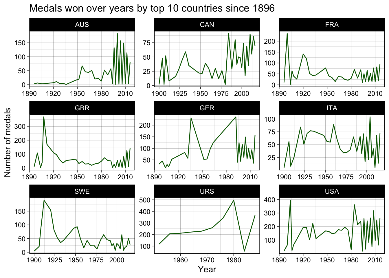

Research Questions

1. Is there an unbiased ranking system to determine the rankings of nations in Olympics? Can we rank different nations on varied ranking systems (different weightage for gold, silver and bronze) and observe how their ranks differ based on weightage given to gold, silver and bronze medals? - Ranking System section
2. Can we identify the most decorated athlete of all time, most decorated men and women athlete? Can we also identify impactful performances of athletes? - Decorated Athletes section
3. Can we identify the age of men and women athletes where their performance is maximized? Does this differ for countries? - Peak Performant Age section
4. Can we identify if there is a correlation of features like height/weight/age to specific sports? (For example if height positively impacts basketball, age helps in shooting or athletics, etc.) Does it equally hold for both the genders? Correlation of features to Sport section

Ranking System

Is there an unbiased ranking system to determine the rankings of nations in Olympics? Can we rank different nations on varied ranking systems (different weightage for gold, silver and bronze) and observe how their ranks differ based on weightage given to gold, silver and bronze medals?

Code

(countries_participated_year <- olympics_data %>%
  distinct(NOC, Year)%>%
  group_by(Year) %>%
  summarise(no_countries_participated = n()) %>%
  arrange(desc(no_countries_participated)))

230 countries participated in Olympics since the start till the event in 2016. So, we will analyse how varied ranking systems for different years(approx two or three years) in which the number of countries participated is greater than 200 to ensure that we find an unbiased ranking system. We will use that system to rank nations for one random year and also over the years.

Design.

The total weighted medal values for each country determine the country’s rank in the Olympics. The weighted value of the medals won by a country is found by multiplying the number of gold, silver and bronze medals by their respective weight and then summing them. Bronze medals are always worth one point. Gold medals can’t be worth less than silver and silver can’t be worth less than bronze.

A ranking system is defined by silver multiplier and gold multiplier (bronze is always worth 1 point).The weighted value for silver in a ranking system is calculated by multiplying the number of silver medals by weight multiplier of silver. The weight for gold in a ranking system is calculated by multiplying the number of gold medals by weight multiplier of gold. Each country’s weighted medal values are summed for each medal. These totals are ranked in such a fashion that the lowest rank is allotted to the country with the highest weighted value.

Description of Ranking Systems used in the analysis. (Each system is defined by silver and gold multiplier)

1. System 1 - Silver multiplier = Gold multiplier = 1. All medals are weighed equally. So, the nations are ranked based on the total medals won.
2. System 2 - Silver multiplier = 2, Gold multiplier = 5.
3. System 3 - Silver multiplier = 5, Gold multiplier = 5.
4. System 4 - Silver multiplier = 2, Gold multiplier = 10.
5. System 5 - Silver multiplier = 5, Gold multiplier = 10.
6. System 6 - Silver multiplier = 5, Gold multiplier = 20.
7. System 7 - Bronze mutliplier = Silver multiplier = 0, Gold multiplier = 1. Only gold medals are important.

I will verify the ranking systems for years 2016 and 2008.

Code

(medals_2016 <- medals %>%
  filter(Year == 2016) %>%
  group_by(NOC, Medal) %>%
  summarise(count = n()) %>%
  pivot_wider(names_from=Medal, values_from=count, values_fill=0) %>%
  ungroup %>%
  mutate(system_1 = Gold + Silver + Bronze,
         rank_1 = min_rank(-system_1),
         system_2 = 5*Gold + 2*Silver + Bronze,
         rank_2 = min_rank(-system_2),
         system_3 = 5*Gold + 5*Silver + Bronze,
         rank_3 = min_rank(-system_3),
         system_4 = 10*Gold + 2*Silver + Bronze,
         rank_4 = min_rank(-system_4),
         system_5 = 10*Gold + 5*Silver + Bronze,
         rank_5 = min_rank(-system_5),
         system_6 = 20*Gold + 5*Silver + Bronze,
         rank_6 = min_rank(-system_6),
         system_7 = Gold,
         rank_7 = min_rank(-system_7)) %>%
   arrange(rank_1))

Code

ranks_2016 <- medals_2016 %>%
  select(NOC, rank_1, rank_2, rank_3, rank_4, rank_5, rank_6, rank_7) %>%
  arrange(rank_1) %>%
  slice(1:50) %>%
  pivot_longer(c("rank_1", "rank_2", "rank_3", "rank_4", "rank_5", "rank_6", "rank_7"),
               names_to = "type",
               values_to = "rank")

ggplot(ranks_2016, aes(x = type, y=NOC, label=rank, fill=rank)) +
  geom_tile() +
  geom_text(color = "white", size = 2)+
  scale_fill_continuous(low = "darkorange",
                        high = "darkblue",
                        name = "rank") +
  scale_x_discrete(labels=c('1:1:1',
                            '5:2:1',
                            '5:5:1',
                            '10:2:1',
                            '10:5:1',
                            '20:5:1',
                            '1:0:0')) +
  theme(axis.text.x = element_text(angle = 90),
        axis.text.y = element_text(size = 6))+
  labs(title = "Heatmap of rankings for top 50 total medal winning countries in 2016",
       subtitle = "X-label represent weight multiplier for each medal type",
       y = "Nation",
       x = "Ranking System (Gold:Silver:Bronze)")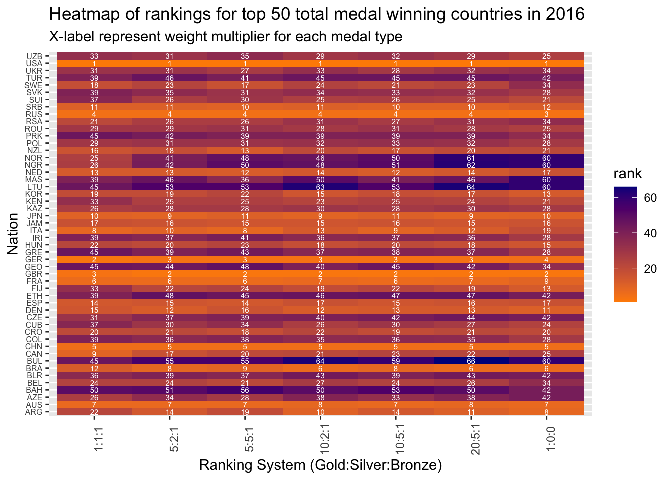

From the above heatmap of rankings for year 2016, we can see that, rank_5 has the least deviation from rankings by other systems for most of the countries. Also, rank_2 is fairly close to most of the other rankings. Hence, either of them can be used as the best estimator of country rankings for the year 2016. Likewise, let’s verify for year 2008 and see if there is a common best system for both the years.

Code

(medals_2008 <- medals %>%
  filter(Year == 2008) %>%
  group_by(NOC, Medal) %>%
  summarise(count = n()) %>%
  pivot_wider(names_from=Medal, values_from=count, values_fill=0) %>%
  ungroup %>%
  mutate(system_1 = Gold + Silver + Bronze,
         rank_1 = min_rank(-system_1),
         system_2 = 5*Gold + 2*Silver + Bronze,
         rank_2 = min_rank(-system_2),
         system_3 = 5*Gold + 5*Silver + Bronze,
         rank_3 = min_rank(-system_3),
         system_4 = 10*Gold + 2*Silver + Bronze,
         rank_4 = min_rank(-system_4),
         system_5 = 10*Gold + 5*Silver + Bronze,
         rank_5 = min_rank(-system_5),
         system_6 = 20*Gold + 5*Silver + Bronze,
         rank_6 = min_rank(-system_6),
         system_7 = Gold,
         rank_7 = min_rank(-system_7)) %>%
   arrange(rank_1))

Code

ranks_2008 <- medals_2008 %>%
  select(NOC, rank_1, rank_2, rank_3, rank_4, rank_5, rank_6, rank_7) %>%
  arrange(rank_1) %>%
  slice(1:50) %>%
  pivot_longer(c("rank_1", "rank_2", "rank_3", "rank_4", "rank_5", "rank_6", "rank_7"),
               names_to = "type",
               values_to = "rank")

ggplot(ranks_2008, aes(x = type, y=NOC, label=rank, fill=rank)) +
  geom_tile() +
  geom_text(color = "white", size = 2)+
  scale_fill_continuous(low = "darkorange",
                        high = "darkblue",
                        name = "rank") +
  scale_x_discrete(labels=c('1:1:1',
                            '5:2:1',
                            '5:5:1',
                            '10:2:1',
                            '10:5:1',
                            '20:5:1',
                            '1:0:0')) +
  theme(axis.text.x = element_text(angle = 90),
        axis.text.y = element_text(size = 6))+
  labs(title = "Heatmap of rankings for top 50 total medal winning countries in 2008",
       subtitle = "X-label represent weight multiplier for each medal type",
       y = "Nation",
       x = "Ranking System (Gold:Silver:Bronze)")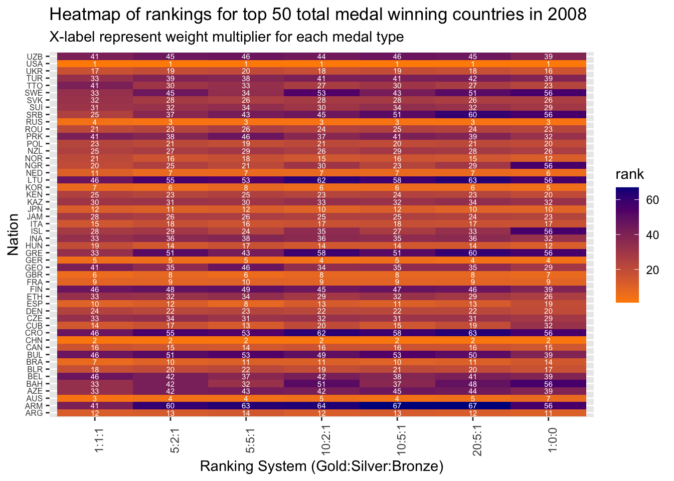

From the above heatmap of rankings for year 2008, we can see that, rank_5 has the least deviation from rankings by other systems for most of the countries. Also, rank_3 is fairly close to most of the other rankings. Hence, either of them can be used as the best estimators of country rankings for the year 2008.

Analysis on 2008 and 2016 showed that ranking system 5 has the least deviation from other rankings. So, we can use this as the best estimator for ranking nations. This might not be completely unbiased but it fairly ranks the countries according to the medals won.

Below table shows rankings of countries for the year 1912 using system 5.

Code

(medals_1912 <- medals %>%
  filter(Year == 1912) %>%
  group_by(NOC, Medal) %>%
  summarise(count = n()) %>%
  pivot_wider(names_from=Medal, values_from=count, values_fill=0) %>%
  ungroup %>%
  mutate(points = 10*Gold + 5*Silver + Bronze,
         rank = min_rank(-points)) %>%
  arrange(rank))

Let’s see the overall rankings from 1896 to 2016 using ranking system 5. We will rank based on average_points per appearance. Total points is divided by number of appearances to eliminate bias (to some extent) that occurs from the fact that a few nations might take part more number of times compared to others. Only nations above 10th percentile of number of appearances are ranked because there could be outliers on the lower end (especially countries who participated only once).

Code

medals_all_years <- medals %>%
  group_by(NOC, Medal) %>%
  summarise(count = n()) %>%
  pivot_wider(names_from=Medal, values_from=count, values_fill=0) %>%
  ungroup %>%
  mutate(points = 10*Gold + 5*Silver + Bronze)

appearances <- olympics_data %>%
  distinct(NOC, Year) %>%
  group_by(NOC) %>%
  summarise(no_appearances = n())

no_appearances_10p <- quantile(appearances$no_appearances, probs = 0.1)

appearances <- appearances %>%
  filter(no_appearances > no_appearances_10p )

medals_all_years <- inner_join(medals_all_years,
                               appearances,
                               by = "NOC") %>%
  mutate(avg_points_per_appearance = points/no_appearances,
         rank = min_rank(-avg_points_per_appearance)) %>%
  arrange(rank)

medals_all_years

Decorated Athletes

Can we identify the most decorated athlete of all time, most decorated men and women athlete?

First we compute the weighted value of medals (points) won by athletes across years using ranking system 5 (the best ranking system as shown previously). The most decorated athlete is definitely based on the number of points earned.

Another points system to rank athletes performance can be designed based on number of events the athlete has participated in years and the number of appearances over years. This ranking can be defined as impact rankings. This system tries to give weightage to closely comparable points based on time frame and participation in number of events(either lesser appearances or lesser events are weighted higher). Impact ranking is based on extrapolated impact points. Impact points are calculated by using points, normalized number of events (normal_events) and normalized number of appearances(normal_years). Only athletes with number of events and number of appearances above 10th percentile are ranked because there could be outliers on the lower end (especially for those who either participated in a single event or only appeared once). \[ impact\_points = (points * normal\_events)/normal\_years \]

Code

athletes_gender <- olympics_data %>%
  distinct(Name, Sex) %>%
  select(Name, Sex)

athlete_medals_all_years <- medals %>%
  group_by(Name, Medal) %>%
  summarise(count = n()) %>%
  ungroup() %>%
  pivot_wider(names_from=Medal, values_from=count, values_fill=0) %>%
  ungroup %>%
  mutate(points = 10*Gold + 5*Silver + Bronze,
         rank_decorated = min_rank(-points))

decorated_rankings <- inner_join(athlete_medals_all_years,
                                 athletes_gender,
                                 by = "Name") %>%
  arrange(rank_decorated)

appearances_years <- olympics_data %>%
  distinct(Name, Year) %>%
  group_by(Name) %>%
  summarise(no_years = n()) %>%
  mutate(normal_years = (no_years - min(no_years))/(max(no_years) - min(no_years)))

no_years_10p <- quantile(appearances_years$no_years, probs = 0.1)

appearances_years <- appearances_years %>%
  filter(no_years > no_years_10p )

appearances_events <- olympics_data %>%
  group_by(Name) %>%
  summarise(no_events = n()) %>%
  mutate(normal_events = (no_events - min(no_events))/(max(no_events) - min(no_events)))

no_events_10p <- quantile(appearances_events$no_events, probs = 0.1)

appearances_events <- appearances_events %>%
  filter(no_events > no_events_10p )

athlete_medals_events_all_years <- inner_join(athlete_medals_all_years,
                               appearances_events,
                               by = "Name")

athlete_medals_events_years <- inner_join(athlete_medals_events_all_years,
                               appearances_years,
                               by = "Name") %>%
  mutate(impact_points = (points * normal_events)/normal_years,
         rank_impact = min_rank(-impact_points)) %>%
  select(-rank_decorated, -normal_events, -normal_years)

impact_rankings <- inner_join(athlete_medals_events_years,
                                 athletes_gender,
                                 by = "Name") %>%
  arrange(rank_impact)

decorated_rankings

Code

impact_rankings

From the above rankings, we can conclude that Michael Fred Phelps, II is the most decorated and impactful player ever in the history of the Olympics. He is also the the most decorated and impactful athlete in men. He won a total of 23 gold, 3 silver and 2 bronze medals in 5 appearances across 30 events. Whereas, Larysa Semenivna Latynina (Diriy-) is the most decorated and impactful women athlete. She won 9 gold, 5 Silver and 4 bronze medals in 3 appearances across 19 events.

Code

ggplot(decorated_rankings, aes(points)) +
  geom_histogram( bins = 60, fill="darkblue") +
  theme_linedraw() +
  facet_wrap(~Sex, scales = "free") +
  labs(title = "Athletes points distribution")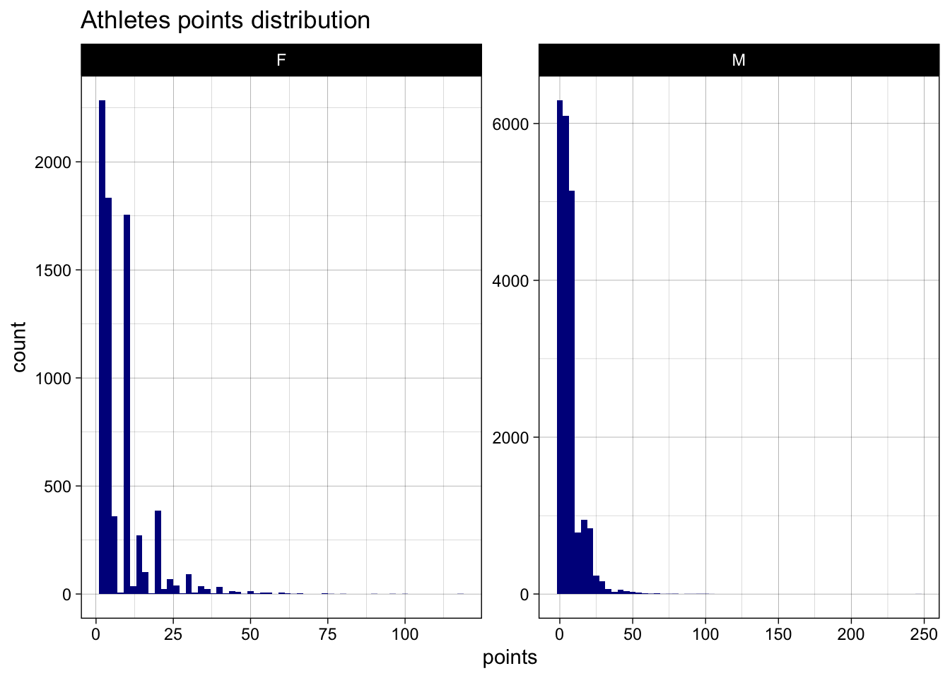

Code

ggplot(impact_rankings, aes(impact_points)) +
  geom_histogram(bins = 60, fill="darkorange") +
  theme_linedraw() +
  facet_wrap(~Sex, scales = "free") +
  labs(title = "Athletes impact points distribution",
       x = "points")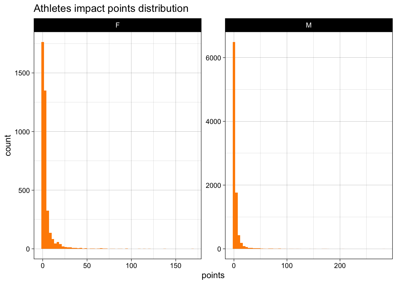

Peak Performant Age

Can we identify the age of men and women athletes where their performance is maximized? Does this differ for countries?

Here we try to identify the age where most of the athletes won medals. This is a direct reflection about the peak performance of an athlete.

Code

olympics_medals_encode <- olympics_data %>%
  mutate(is_medal_won = case_when(
         Medal == "Gold" | Medal == "Silver" | Medal == "Bronze" ~ "medal",
         TRUE ~ "no_medal"))

age_wise_medals <-  olympics_medals_encode%>%
  filter(!is.na(Age)) %>%
  group_by(Sex, Age, is_medal_won) %>%
  summarise(no_medals = n())

ggplot(age_wise_medals, aes(x=Age, y=no_medals, size = no_medals,color=is_medal_won)) +
  geom_point(alpha=0.6) +
  scale_size(range = c(.1, 10), name="Medals")+
  theme_linedraw()+
  facet_wrap(vars(Sex),nrow=2, ncol=1) +
  labs(title = "Scatter plot for medals won vs age",
       subtitle = "Size of bubble represents number of medals won",
       x = "age",
       y = "Number of Medals",
       color = "Position")+
  theme(legend.position = "top")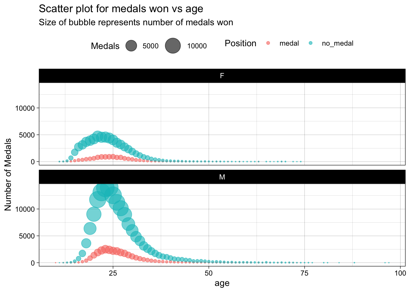

From the above visualizations, we can conclude that peak performant age for male athletes is between 22 to 24 . While for females, it is between 23 to 26. This prediction is also evident from the raw data shown in the following tables.

Code

(age_wise_medals %>%
  filter(Sex == "M",
         is_medal_won == "medal") %>%
  arrange(desc(no_medals)) %>%
  select(-is_medal_won))

Code

(age_wise_medals %>%
  filter(Sex == "F",
         is_medal_won == "medal") %>%
  arrange(desc(no_medals)) %>%
  select(-is_medal_won))

Code

age_top10_country_wise_medals <- olympics_data %>%
  filter(NOC %in% teams_medals_total[1:10,]$NOC) %>%
  mutate(is_medal_won = case_when(
         Medal == "Gold" | Medal == "Silver" | Medal == "Bronze" ~ "medal",
         TRUE ~ "no_medal")
  ) %>%
  filter(!is.na(Age), is_medal_won == "medal") %>%
  group_by(Sex, NOC, Age) %>%
  summarise(no_medals = n())

ggplot(age_top10_country_wise_medals, aes(x=reorder(NOC, Age, mean), y=Age, fill=Sex)) +
  geom_jitter(color="black",size=0.2) +
  geom_boxplot(varwidth = TRUE, alpha = 0.5) +
  scale_size(range = c(.1, 10), name="Medals")+
  theme_linedraw()+
  facet_wrap(~Sex, ncol=1, scales = "free_y") +
  labs(title = "Ages of athletes - Top 10 medal winning nations",
       x = "NOC",
       y = "Age")+
  theme(legend.position = "none")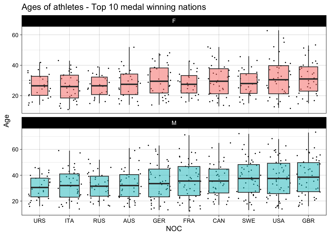

Code

(age_top10_country_wise_medals %>%
  group_by(Sex, NOC) %>%
  summarise(mean_age = mean(Age),
            median_age = median(Age)) %>%
  arrange(Sex,mean_age))

From the above graphs and table we can see that the mean medal winning age is different for different countries. Italy has the least mean for medal winning age in females and Soviet Union(URS) has the least in males. We can say that this difference might be present because of differences in a few influential attributes like body type, difference in nutrition habits across countries and the way they train.

Correlation of features to Sport

Can we identify if there is a correlation of features like height/weight/age to specific sports? Does it equally hold for both the genders?

I will be analyzing height for basketball, age for athletics and shooting. We can’t verify traits like height, weight for athletics because it has variety of events where same trait might not be significant. Whereas in shooting, I believe age matters the most because we can make an assessment on concentration levels which is key to this sport.

Code

basketball_medals <-  olympics_medals_encode%>%
  filter(Sport == "Basketball", !is.na(Height)) %>%
  group_by(Sex, Height, is_medal_won) %>%
  summarise(no_medals = n())

ggplot(basketball_medals,
       aes(x=Height, y=no_medals, size = no_medals, color=is_medal_won)) +
  geom_point(alpha=0.6) +
  scale_size(range = c(.1, 10), name="Medals")+
  theme_linedraw()+
  facet_wrap(vars(Sex), nrow = 2, ncol = 1) +
  labs(title = "Scatter plot for medals won vs height in basketball",
       subtitle = "Size of bubble represents number of medals won",
       x = "height",
       y = "Number of Medals",
       color = "Position")+
  theme(legend.position = "top")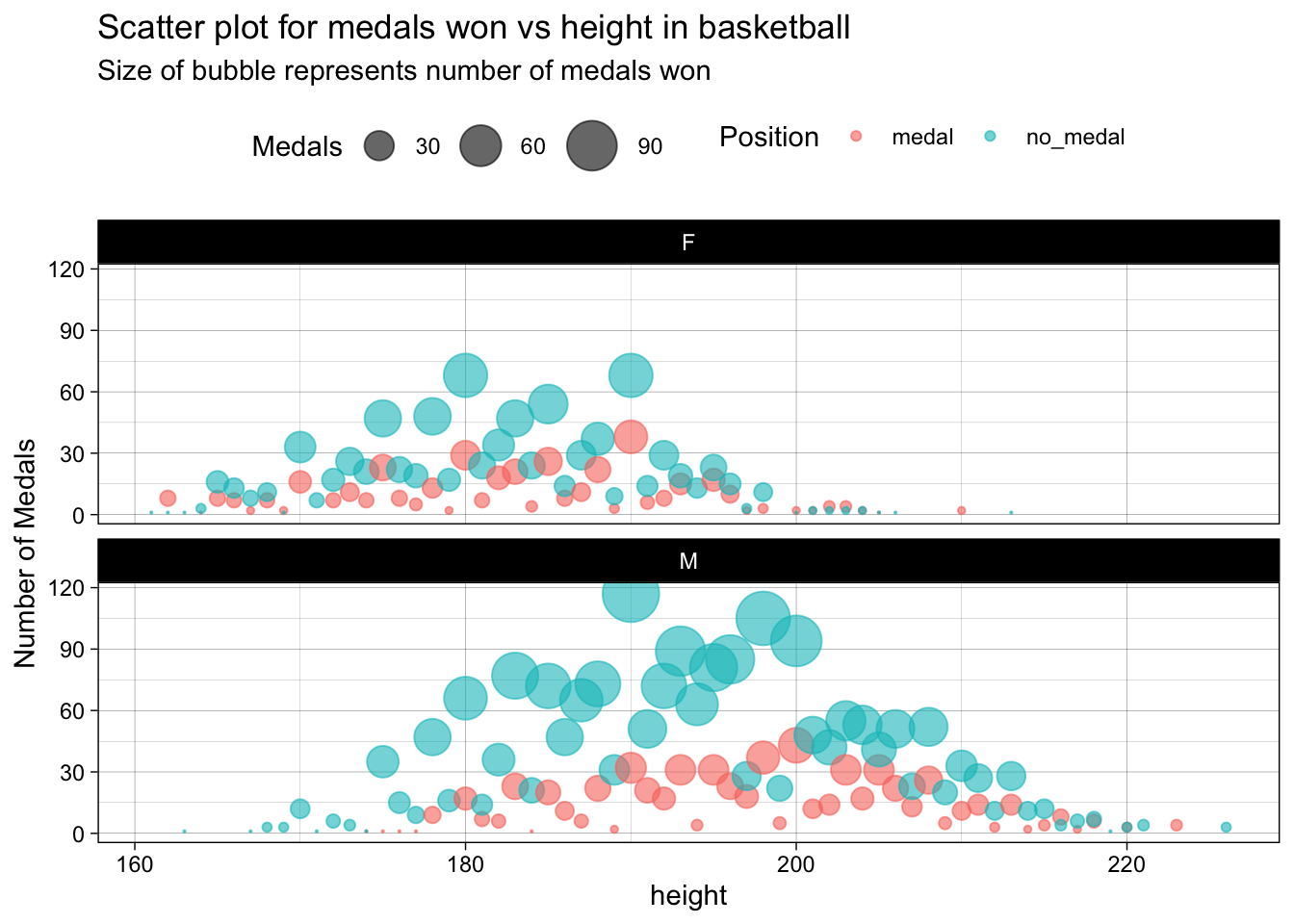

For basketball, men with height ranging from 190 to 205 cm have won most of the medals. For females, it is between 180 to 190 cm. So, we can say that height has a positive affect on winning in basketball because majority of the medal winning athletes are tall.

Code

athletics_medals <-  olympics_medals_encode%>%
  filter(Sport == "Athletics", !is.na(Age)) %>%
  group_by(Sex, Age, is_medal_won) %>%
  summarise(no_medals = n())

ggplot(athletics_medals,
       aes(x=Age, y=no_medals, size = no_medals, color=is_medal_won)) +
  geom_point(alpha=0.6) +
  scale_size(range = c(.1, 10), name="Medals")+
  theme_linedraw()+
  facet_wrap(vars(Sex), nrow = 2, ncol = 1) +
  labs(title = "Scatter plot for medals won vs age in athletics",
       subtitle = "Size of bubble represents number of medals won",
       x = "age",
       y = "Number of Medals",
       color = "Position")+
  theme(legend.position = "top")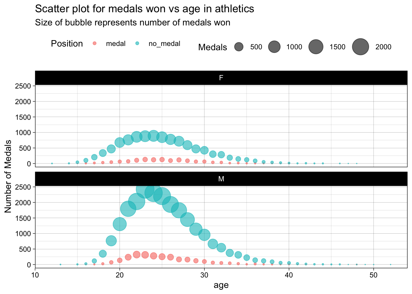

In athletics, for both the genders most of the medals winners are between ages 20 and 30. Also, we can observe that most of the participants age is also in this bracket. We can say that since this is the age with maximum potential of human body, age factor is dominant in athletics.

Code

shooting_medals <-  olympics_medals_encode%>%
  filter(Sport == "Shooting", !is.na(Age)) %>%
  group_by(Sex, Age, is_medal_won) %>%
  summarise(no_medals = n())

ggplot(shooting_medals,
       aes(x=Age, y=no_medals, size = no_medals, color=is_medal_won)) +
  geom_point(alpha=0.6) +
  scale_size(range = c(.1, 10), name="Medals")+
  theme_linedraw()+
  facet_wrap(vars(Sex), nrow = 2, ncol = 1) +
  labs(title = "Scatter plot for medals won vs age in shooting",
       subtitle = "Size of bubble represents number of medals won",
       x = "age",
       y = "Number of Medals",
       color = "Position")+
  theme(legend.position = "top")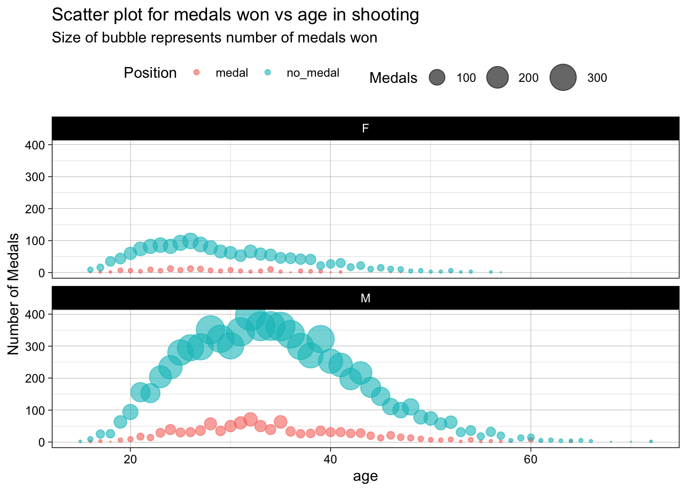

In shooting, for both the genders most of the medals winners are between 20 and 40. We can claim that this is the age with maximum potential of human body and the concentrations levels are higher in the younger age. So, age factor is dominant in shooting.

Conclusion

1. The number of athletes, events, and participating nations has grown dramatically since 1896.

2. We have identified that ranking system 5 is the closest to an unbiased system. In this system we use 10, 5 and 1 weights for gold, silver and bronze respectively.

3. Michael Fred Phelps, II is the most decorated male athlete and Larysa Semenivna Latynina (Diriy-) is the most decorated female athlete. Phelps won 23 gold, 3 silver and 2 bronze in 5 appearances. Larysa Semenivna Latynina (Diriy-) won 9 gold, 5 Silver and 4 bronze medals in 3 appearances. They are also the most impactful athletes ever.

4. Peak performance age for male athletes is between 22 to 24 and for females it is between 23 to 26. Also the mean age of medal winners is different across nations.

5. We observed significance of traits like height/age in sports and the data supports it. So, height matters in basketball and age matters in both athletics and shooting.

Limitiations

1. It is quite tough to identify decorated/impactful athletes just from visualizations.
2. Identifying the best ranking systems from heatmap could be challenging for general audience. But can be done.
3. In the treemap showing “Sport size proportional to number of events in in Olympics” the labels in the right bottom corner couldn’t be shown because of the sizes of the boxes and this is a bug in treemap library.

Bibliography

Samruddhi Mhatre. “Olympics Dataset (1896 to 2016)” Kaggle, https://www.kaggle.com/datasets/samruddhim/olympics-althlete-events-analysis

Wikipedia - https://en.wikipedia.org/wiki/Olympic_Games

R Core Team (2023). R: A Language and Environment for Statistical Computing. R Foundation for Statistical Computing, Vienna, Austria. https://www.R-project.org/.

Wickham, Hadley, et al. R for Data Science: Import, Tidy, Transform, Visualize, and Model Data. 2nd ed., O’Reilly Media, Inc, 2023. http://r4ds.hadley.nz/