Week 2 Challenge

Claire Battaglia

challenge2

Author

Claire Battaglia

Published

March 1, 2023

Code

library(tidyverse)
library(igraph)
library(statnet)

knitr::opts_chunk$set(echo = TRUE)

Describe the network data

This week I’ll be creating a network of the distances between various places in Game of Thrones. The data are organized in an edgelist.

Code

# read in data
dist <- read_csv("_data/got/got_distances.csv", show_col_types = FALSE)

# reorder columns
dist <- dist %>%
    relocate(From, To, Miles, Mode, .before = "Region From")

# preview
head(dist, 10)

# A tibble: 10 × 6
   From          To               Miles Mode  `Region From` Notes   
   <chr>         <chr>            <dbl> <chr> <chr>         <chr>   
 1 Casterly Rock the Golden Tooth   240 land  Westerlands   <NA>    
 2 Casterly Rock Lannisport          40 land  Westerlands   <NA>    
 3 Casterly Rock Kayce              100 land  Westerlands   <NA>    
 4 Casterly Rock Kayce               12 water Westerlands   <NA>    
 5 Casterly Rock Deep Den           240 land  Westerlands   Goldroad
 6 Deep Den      King’s Landing     590 land  Westerlands   Goldroad
 7 Kayce         Faircastle         480 raven Westerlands   <NA>    
 8 Faircastle    the Crag           115 Boat  Westerlands   Island  
 9 the Crag      Ashemark            85 land  Westerlands   <NA>    
10 Ashemark      Casterly Rock      170 land  Westerlands   <NA>

The “from” and “to” fields are already clearly defined and it seems as though the miles and mode are edge attributes. I’m not sure what the “Region From” field is in the context of a network, though.

Code

# create network object
dist.ig <- graph_from_data_frame(dist, directed = FALSE)

# view
print(dist.ig)

IGRAPH 0440fcf UN-- 134 200 -- 
+ attr: name (v/c), Miles (e/n), Mode (e/c), Region From (e/c), Notes
| (e/c)
+ edges from 0440fcf (vertex names):
 [1] Casterly Rock--the Golden Tooth Casterly Rock--Lannisport      
 [3] Casterly Rock--Kayce            Casterly Rock--Kayce           
 [5] Casterly Rock--Deep Den         Deep Den     --King’s Landing  
 [7] Kayce        --Faircastle       Faircastle   --the Crag        
 [9] the Crag     --Ashemark         Casterly Rock--Ashemark        
[11] Ashemark     --the Golden Tooth Lannisport   --Crakehall       
[13] Crakehall    --Old Oak          Old Oak      --Highgarden      
+ ... omitted several edges

We can see a few things from this summary:

The network is undirected. This makes sense as distances between physical locations are by nature symmetrical.
The network is named. I.e. the nodes/vertices have names. In this network the nodes are physical places with names.
The edges are unweighted.
It is not bipartite.
There are 134 nodes/vertices.
There are 200 edges/ties.

We can get a bit more information about the nodes and edges.

Code

# get count
vcount(dist.ig)

[1] 134

Code

ecount(dist.ig)

[1] 200

Code

# get attributes
vertex_attr_names(dist.ig)

[1] "name"

Code

edge_attr_names(dist.ig)

[1] "Miles"       "Mode"        "Region From" "Notes"

The “Region From” field is currently being understood as an edge attribute, which doesn’t really make sense to me so I am wondering if I need to specify it as something else.

Dyad and triad census

We can also use a dyad and triad census to get a better understanding of the network.

Code

# dyad census
igraph::dyad.census(dist.ig)

$mut
[1] 190

$asym
[1] 0

$null
[1] 8721

I’m not sure what to make of the dyad census. Given that distances between places are by nature reciprocal, I don’t understand why all the dyads aren’t mutual. There is no way for Casterly Rock to be 240 miles from the Golden Tooth without the Golden Tooth also being 240 miles from Casterly Rock.

Given the number of null dyads (i.e. missing ties), it seems as though the mileage between many places hasn’t been recorded. Again, there is by definition a distance between any two physical places.

Code

# triad census
igraph::triad.census(dist.ig)

Warning in igraph::triad.census(dist.ig): At core/misc/motifs.c:1165 : Triad
census called on an undirected graph.

 [1] 368822      0  22731      0      0      0      0      0      0      0
[11]    501      0      0      0      0     30

A triad census doesn’t work on an undirected grapgh so I’m not sure whether there is anything meaningful here.

Logically we know there is a distance between every two physical place so it seems like the dyad and triad census in this case is more useful for revealing missing distances than anything else.

If the ties in this network were roads or established routes of some kind, both censuses could reveal interesting insight into places that are more connected than others but distance is a feature of the physical world, not a human creation.

Global and local transitivity

Code

# get global trans
transitivity(dist.ig)

[1] 0.1522843

Code

# get avg local trans
transitivity(dist.ig, type = "average")

[1] 0.1767116

Code

# get local trans of Winterfell, Casterly Rock
transitivity(dist.ig, type = "local", vids = V(dist.ig)[c("Winterfell", "Casterly Rock")])

[1] 0.03571429 0.09523810

We can see that the transitivity scores of Winterfell and Casterly Rock are .04 and .1, respectively, indicating that in the context of this network, a higher percentage of the nodes connected to Casterly Rock are also connected to each other than for Winterfell.

Again, the concept of transitivity doesn’t make a lot of sense when we’re talking about distances between physical features.

Path length and component structure

Code

# get component names
names(igraph::components(dist.ig))

[1] "membership" "csize"      "no"

Code

# get number of components
igraph::components(dist.ig)$no

[1] 3

Code

# get size of components
igraph::components(dist.ig)$csize

[1] 129   3   2

This is interesting. There are three components in the network. If the network included the distances between each of the places included—as in a map—there would be just a single component in the network. Either the network is missing a lot of information or I read it in incorrectly.

Code

# get distance between Winterfell and Casterly Rock
distances(dist.ig,"Winterfell","Casterly Rock")

           Casterly Rock
Winterfell             2

Code

# get distance between Winterfell and King’s Landing
distances(dist.ig,"Winterfell","King’s Landing")

           King’s Landing
Winterfell              1

Code

# get distance between Casterly Rock and King’s Landing
distances(dist.ig,"King’s Landing","Casterly Rock")

               Casterly Rock
King’s Landing             1

Both Winterfell and Casterly Rock are equidistant from King’s Landing. We know this isn’t true in terms of the number of miles so I think this is talking about the number of nodes in between each of them and King’s Landing. This is interesting because even this measure of distance (i.e. number of nodes instead of number of miles) can have profound socio-political implications.

Code

# get density
graph.density(dist.ig, loops = T)

[1] 0.02211166

Code

# remove multiple and loops
dist.ig <- simplify(dist.ig, remove.multiple = F, remove.loops = T)

# assign weight??
#E(dist.ig)$weight <- E(dist.ig)$Miles

# plot network
plot(dist.ig,
     vertex.size = 5,
     vertex.color = "maroon",
     vertex.label.cex = .5,
     main = "Distances between places in Game of Thrones")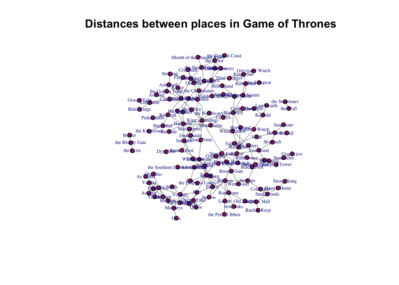

Questions

What to do with “Region From” field? This is potentially meaningful information but I’m not sure how to incorporate it into the network.
How to make the length of the tie proportional to the number of miles? I’d like the distance() function to return the number of miles between two nodes–is this possible?
How to display the number of miles?
How to color the edges according to the mode?