# Datasetdf <- CollegePlaying#First 6 rows of the datasetkable(head(df),caption ="First 6 rows of Dataset")
First 6 rows of Dataset
playerID
schoolID
yearID
aardsda01
pennst
2001
aardsda01
rice
2002
aardsda01
rice
2003
abadan01
gamiddl
1992
abadan01
gamiddl
1993
abbeybe01
vermont
1889
Constructing Network
Code
# years having attended more than 300ylist <-c(1985,1986,1987,1988,1989,1990)g <-graph.data.frame(df[df$yearID %in% ylist,],directed = T)V(g)$type <-V(g)$name %in% df[df$yearID %in% ylist,1]g
# GEt the largest componentcomponents <-clusters(g, mode="weak")biggest_cluster_id <-which.max(components$csize)# idsvert_ids <-V(g)[components$membership == biggest_cluster_id]# subgraphg <-induced_subgraph(g, vert_ids)
Network Plot
Code
grp <-ifelse(V(g)$type,"Player","School")nodes <-data.frame(id =V(g)$name, title =V(g)$name, group = grp)edges <-get.data.frame(g, what="edges")[1:2]vis.nodes <- nodesvis.links <- edges#giving some styles to nodes and edgesvis.nodes$shadow <-TRUE# Nodes will drop shadowvis.nodes$label <- vis.nodes$id # Node labelvis.nodes$size <-degree(g)+20# Node sizevis.nodes$borderWidth <-2# Node border widthvis.links$color <-"gray"# line color vis.links$smooth <-FALSE# should the edges be curved?vis.links$shadow <-FALSE# edge shadowvisnet3 =visNetwork(vis.nodes, vis.links, main ="Network of Player Attending School") %>%visPhysics(solver ="forceAtlas2Based",forceAtlas2Based =list(gravitationalConstant =-100))visLegend(visnet3,main ="Groups")
Network Stats
Code
################################## Network Stats ##################################mx_cliq <-clique.number(g)k <-data.frame(Measure =c("Nodes","Edges","Radius","Diameter","Reciprocity","Average Degree","Density","Number of Clusters","Largest Clique Size","Number of Largest Cliques","Average Shortest Path","Clustering Coefficient","Number of Cores","Number of Triangles"),Value =c(vcount(g),ecount(g),radius(g),diameter(g),reciprocity(g),mean(degree(g,mode ="all")),graph.density(g),clusters(g)$no,mx_cliq,length(cliques(as.undirected(g),min = mx_cliq)),average.path.length(g),transitivity(g),length(unique(coreness(g))),length(triangles(g))))k$Value <-round(k$Value,5)kable(k,caption ="Player's Atending School Network Stats")
wk <-walktrap.community(g)grp <- wk$membershipnodes <-data.frame(id =V(g)$name, title =V(g)$name, group = grp)edges <-get.data.frame(g, what="edges")[1:2]vis.nodes <- nodesvis.links <- edges#giving some styles to nodes and edgesvis.nodes$shadow <-TRUE# Nodes will drop shadowvis.nodes$label <- vis.nodes$id # Node labelvis.nodes$size <-degree(g)+20# Node sizevis.nodes$borderWidth <-2# Node border widthvis.links$color <-"gray"# line color vis.links$smooth <-FALSE# should the edges be curved?vis.links$shadow <-FALSE# edge shadowvisnet3 =visNetwork(vis.nodes, vis.links, main ="Walk Trap : Network of Player Attending School") %>%visPhysics(solver ="forceAtlas2Based",forceAtlas2Based =list(gravitationalConstant =-100))visLegend(visnet3,main ="Communities")
Call:
ergm(formula = g ~ edges + nodecov("Eigen") + nodecov("Degree"))

Maximum Likelihood Results:

                Estimate Std. Error MCMC % z value Pr(>|z|)
edges          -6.568340   0.101491      0 -64.718   <1e-04 ***
nodecov.Eigen  -1.167338   0.275706      0  -4.234   <1e-04 ***
nodecov.Degree  0.097185   0.004308      0  22.557   <1e-04 ***
---
Signif. codes:  0 '***' 0.001 '**' 0.01 '*' 0.05 '.' 0.1 ' ' 1

     Null Deviance: 82873  on 59780  degrees of freedom
 Residual Deviance:  2860  on 59777  degrees of freedom

AIC: 2866  BIC: 2893  (Smaller is better. MC Std. Err. = 0)
Code
# the odds ratio for each term. or <-exp(coef(m1))
CUG test
Code
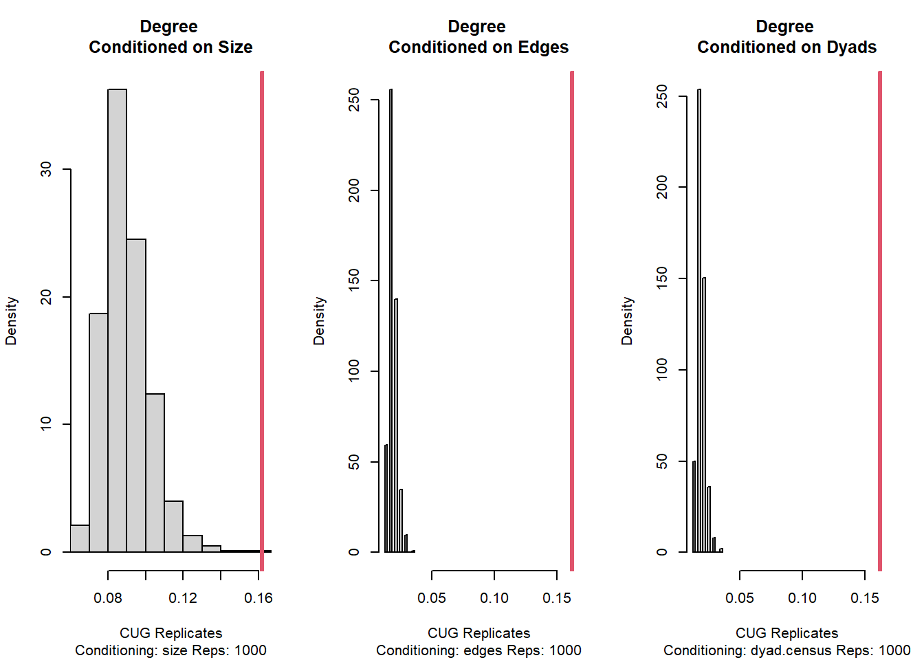
#CuG test on the network using mode sizectest <-cug.test(g, centralization,FUN.arg=list(FUN=degree), mode="graph", cmode="size")#CuG test on the network using mode dyad.censusctest2 <-cug.test(g, centralization,FUN.arg=list(FUN=degree), mode="graph", cmode="dyad.census")#CuG test on the network using mode edgesctest3 <-cug.test(g, centralization,FUN.arg=list(FUN=degree), mode="graph", cmode="edges")par(mfrow=c(1,3))plot(ctest, main="Degree \nConditioned on Size" )plot(ctest3, main="Degree \nConditioned on Edges" )plot(ctest2, main="Degree \nConditioned on Dyads" )
Code
par(mfrow=c(1,1))
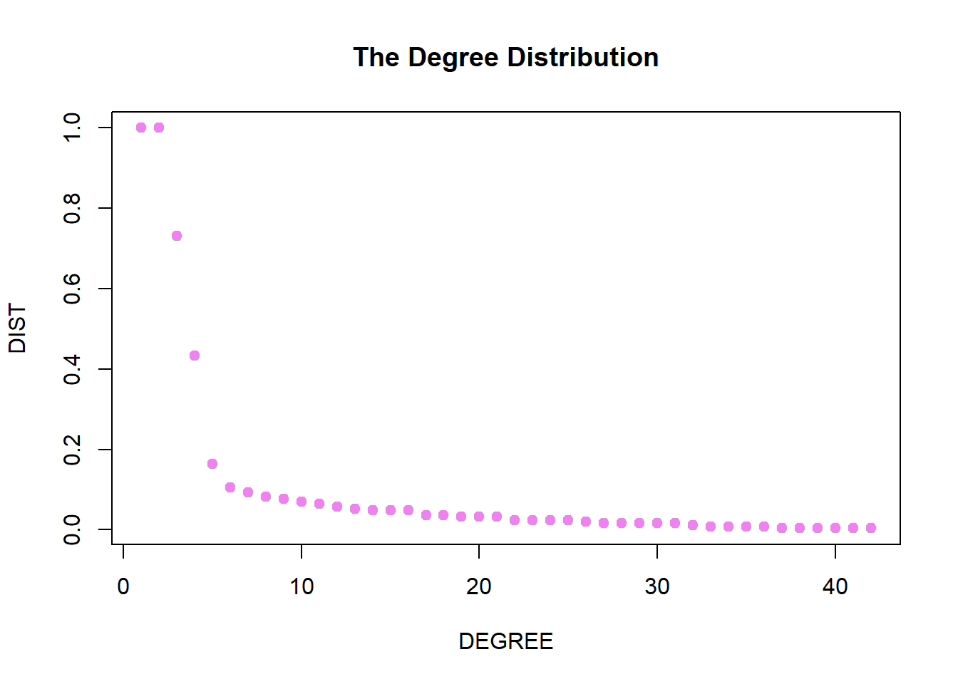
Source Code
---title: 'Bipartite Network Analysis: Players Attending School'author: "Amer Abuhasan"description: "Final Project"date: "05/12/2023"format: html: toc: true code-fold: true code-copy: true code-tools: truecategories: - Final Project - Amer Abuhasan ---```{r}#| label: setup#| include: falseknitr::opts_chunk$set(echo =TRUE, warning=FALSE,message=FALSE)library(Lahman)library(igraph)library(visNetwork)library(knitr)```# Reading Data```{r}# Datasetdf <- CollegePlaying#First 6 rows of the datasetkable(head(df),caption ="First 6 rows of Dataset")```# Constructing Network```{r}# years having attended more than 300ylist <-c(1985,1986,1987,1988,1989,1990)g <-graph.data.frame(df[df$yearID %in% ylist,],directed = T)V(g)$type <-V(g)$name %in% df[df$yearID %in% ylist,1]g```## Get the Largest Component```{r}# GEt the largest componentcomponents <-clusters(g, mode="weak")biggest_cluster_id <-which.max(components$csize)# idsvert_ids <-V(g)[components$membership == biggest_cluster_id]# subgraphg <-induced_subgraph(g, vert_ids)```# Network Plot```{r}grp <-ifelse(V(g)$type,"Player","School")nodes <-data.frame(id =V(g)$name, title =V(g)$name, group = grp)edges <-get.data.frame(g, what="edges")[1:2]vis.nodes <- nodesvis.links <- edges#giving some styles to nodes and edgesvis.nodes$shadow <-TRUE# Nodes will drop shadowvis.nodes$label <- vis.nodes$id # Node labelvis.nodes$size <-degree(g)+20# Node sizevis.nodes$borderWidth <-2# Node border widthvis.links$color <-"gray"# line color vis.links$smooth <-FALSE# should the edges be curved?vis.links$shadow <-FALSE# edge shadowvisnet3 =visNetwork(vis.nodes, vis.links, main ="Network of Player Attending School") %>%visPhysics(solver ="forceAtlas2Based",forceAtlas2Based =list(gravitationalConstant =-100))visLegend(visnet3,main ="Groups")```# Network Stats```{r}################################## Network Stats ##################################mx_cliq <-clique.number(g)k <-data.frame(Measure =c("Nodes","Edges","Radius","Diameter","Reciprocity","Average Degree","Density","Number of Clusters","Largest Clique Size","Number of Largest Cliques","Average Shortest Path","Clustering Coefficient","Number of Cores","Number of Triangles"),Value =c(vcount(g),ecount(g),radius(g),diameter(g),reciprocity(g),mean(degree(g,mode ="all")),graph.density(g),clusters(g)$no,mx_cliq,length(cliques(as.undirected(g),min = mx_cliq)),average.path.length(g),transitivity(g),length(unique(coreness(g))),length(triangles(g))))k$Value <-round(k$Value,5)kable(k,caption ="Player's Atending School Network Stats")```## Degree Distibution```{r}#plot(degree.distribution(g), col="red") #Plot degree distributionddist <-degree_distribution(g, mode="all", cumulative=TRUE)plot(ddist,col="violet",xlab="DEGREE",ylab="DIST", main="The Degree Distribution", pch=19)```# Community Detection```{r}wk <-walktrap.community(g)grp <- wk$membershipnodes <-data.frame(id =V(g)$name, title =V(g)$name, group = grp)edges <-get.data.frame(g, what="edges")[1:2]vis.nodes <- nodesvis.links <- edges#giving some styles to nodes and edgesvis.nodes$shadow <-TRUE# Nodes will drop shadowvis.nodes$label <- vis.nodes$id # Node labelvis.nodes$size <-degree(g)+20# Node sizevis.nodes$borderWidth <-2# Node border widthvis.links$color <-"gray"# line color vis.links$smooth <-FALSE# should the edges be curved?vis.links$shadow <-FALSE# edge shadowvisnet3 =visNetwork(vis.nodes, vis.links, main ="Walk Trap : Network of Player Attending School") %>%visPhysics(solver ="forceAtlas2Based",forceAtlas2Based =list(gravitationalConstant =-100))visLegend(visnet3,main ="Communities")```# Centralities ```{r}Top10Schools_Degree <-names(sort(degree(g, mode ="in"),decreasing = T))[1:10]Top10Players_Degree <-names(sort(degree(g, mode ="out"),decreasing = T))[1:10]Top10_Bonachic <-names(sort(power_centrality(g),decreasing = T))[1:10]Top10_Eigen <-names(sort(eigen_centrality(g)$vector,decreasing = T))[1:10]Top10_Betweenness <-names(sort(betweenness(as.undirected(g)),decreasing = T))[1:10]df <-data.frame(Top10Schools_Degree, Top10Players_Degree, Top10_Bonachic, Top10_Eigen, Top10_Betweenness)kable(df,caption ="Top 10 nodes (Players & Schools) by Centralities")#Top 10 Schools with value by Degreesort(degree(g, mode ="in"),decreasing = T)[1:10]#Top 10 Players with value by Degreesort(degree(g, mode ="out"),decreasing = T)[1:10]#Top Nodes with values by Bonachic Centralitysort(power_centrality(g),decreasing = T)[1:10]#Top 10 Nodes with values by Eigensort(eigen_centrality(g)$vector,decreasing = T)[1:10]#Top 10 Nodes with values by Betweennesssort(betweenness(as.undirected(g)),decreasing = T)[1:10]```# Network models ```{r, include=FALSE}V(g)$Degree <-degree(g)V(g)$Eigen <-eigen_centrality(g)$vectorV(g)$Com <- wk$membershiprg <-sample_gnp(n=245, p=0.00721)detach(package:igraph)library(sna)library(intergraph)library(ergm)library(statnet)``````{r}g <-asNetwork(g)#basic ERGM modelm <-ergm(g ~ edges)summary(m)#with node level attributesm1 <-ergm(g ~ edges +nodecov("Eigen") +nodecov("Degree")) summary(m1)# the odds ratio for each term. or <-exp(coef(m1)) ```# CUG test```{r}#CuG test on the network using mode sizectest <-cug.test(g, centralization,FUN.arg=list(FUN=degree), mode="graph", cmode="size")#CuG test on the network using mode dyad.censusctest2 <-cug.test(g, centralization,FUN.arg=list(FUN=degree), mode="graph", cmode="dyad.census")#CuG test on the network using mode edgesctest3 <-cug.test(g, centralization,FUN.arg=list(FUN=degree), mode="graph", cmode="edges")par(mfrow=c(1,3))plot(ctest, main="Degree \nConditioned on Size" )plot(ctest3, main="Degree \nConditioned on Edges" )plot(ctest2, main="Degree \nConditioned on Dyads" )par(mfrow=c(1,1))```