Migration Networks

Final Project

Mekhala Kumar

Indian Census data

Internal Migration

final project

Author

Mekhala Kumar

Published

May 22, 2023

Code

library(tidyverse)
library(readxl)
library(ggplot2)
library(plotly)
library(igraph)
library(statnet)
library(reshape2)
library(GGally)
library(ggnetwork)
knitr::opts_chunk$set(echo = TRUE, warning=FALSE, message=FALSE)

Network Analysis of Internal Migration: Unravelling Work and Marriage Migration Patterns in India

Dataset for the Project

The Indian Census collects information about demographics such as population, education levels, languages spoken and migration. It is collected once in every ten years and the latest one was collected in 2011. The data collection for the 2021 round has not been collected yet due to the Coronavirus pandemic (Bharadwaj & Batra, 2022).

For this project, the dataset utilised is the Indian Census Migration Data for the year 2011 (Table D03). I chose the dataset labelled as India which contains information on a state-wise/union-territory-wise level.

In this project, I limited my analysis to internal migration, that is, movement of people to different states/union territories within India. The Indian Census has two definitions of migrants:

Migrant by birth place: This is a person whose enumeration occurs in a place that is not their birthplace (Government of India, n.d.).

Migrant by place of residence: This is a person whose place of enumeration in the current Census is different from the residence they were enumerated in during the last Census (Government of India, n.d.).

Table D03 uses the second definition, it also includes information about the number of years they have resided in the area and reasons why they migrated.

In the Data Science Fundamentals course (DACSS601), I studied reasons people migrated to Bangalore. For this project, I wanted to explore reasons people migrated at the country level, which can be studied through a network. I limited my analysis to two reasons: movement for work and marriage.

Note

I also wanted to note that I took the proportion of migrants that moved from State 1 to State 2 for a particular reason of migration. In further detail, I calculated the proportion by dividing the number of people who moved from State 1 to State 2 for a particular reason by the total number of people who moved from State 1 to State 2. For example, if 5 million people moved from Maharashtra to Karnataka for work and the total number of people who moved was 10 million, then the proportion would be 50%. This was done to control for population bias because certain states send or receive more people simply due to them having a higher population. I noticed this when I created a network based on actual population numbers. It showed Uttar Pradesh as one of the top sending states for various reasons of migration but it was not meaningful since this is the most populated state of India.

Research Question

To study whether there are different internal migration patterns associated with movement for work and movement for marriage.

Reading in the Data

The first few rows and last few rows are unnecessary so they have been removed.

Code

mig_india <- read_excel("_data/Mekhala_data/DS-0000-D03-MDDS.XLSX",skip=5,col_names=c("tab_name","state_code","dist_code","area","res","res_time","last_res","last_res_type","tot_t","tot_m","tot_f","work_t","work_m","work_f","busi_t","busi_m","busi_f","educ_t","educ_m","educ_f","mar_t","mar_m","mar_f","afterbirth_t","afterbirth_m","afterbirth_f","withhh_t","withhh_m","withhh_f","others_t","others_m","others_f"))
dim(mig_india)

[1] 67503    32

Code

head(mig_india)

# A tibble: 6 × 32
  tab_name state_code dist_code area  res   res_time      last_res last_res_type
  <chr>    <chr>      <chr>     <chr> <chr> <chr>         <chr>    <chr>        
1 D0603    00         000       INDIA Total All duration… Total    Total        
2 D0603    00         000       INDIA Total All duration… Last re… Total        
3 D0603    00         000       INDIA Total All duration… Last re… Rural        
4 D0603    00         000       INDIA Total All duration… Last re… Urban        
5 D0603    00         000       INDIA Total All duration… Within … Total        
6 D0603    00         000       INDIA Total All duration… Within … Rural        
# ℹ 24 more variables: tot_t <dbl>, tot_m <dbl>, tot_f <dbl>, work_t <dbl>,
#   work_m <dbl>, work_f <dbl>, busi_t <dbl>, busi_m <dbl>, busi_f <dbl>,
#   educ_t <dbl>, educ_m <dbl>, educ_f <dbl>, mar_t <dbl>, mar_m <dbl>,
#   mar_f <dbl>, afterbirth_t <dbl>, afterbirth_m <dbl>, afterbirth_f <dbl>,
#   withhh_t <dbl>, withhh_m <dbl>, withhh_f <dbl>, others_t <dbl>,
#   others_m <dbl>, others_f <dbl>

Code

tail(mig_india)

# A tibble: 6 × 32
  tab_name      state_code dist_code area  res   res_time last_res last_res_type
  <chr>         <chr>      <chr>     <chr> <chr> <chr>    <chr>    <chr>        
1 D0603         35         000       Stat… Urban Duratio… Countri… Total        
2 D0603         35         000       Stat… Urban Duratio… Other C… Total        
3 D0603         35         000       Stat… Urban Duratio… Unclass… Total        
4 <NA>          <NA>       <NA>      <NA>  <NA>  <NA>     <NA>     <NA>         
5 Note:    1. … <NA>       <NA>      <NA>  <NA>  <NA>     <NA>     <NA>         
6 2. The place… <NA>       <NA>      <NA>  <NA>  <NA>     <NA>     <NA>         
# ℹ 24 more variables: tot_t <dbl>, tot_m <dbl>, tot_f <dbl>, work_t <dbl>,
#   work_m <dbl>, work_f <dbl>, busi_t <dbl>, busi_m <dbl>, busi_f <dbl>,
#   educ_t <dbl>, educ_m <dbl>, educ_f <dbl>, mar_t <dbl>, mar_m <dbl>,
#   mar_f <dbl>, afterbirth_t <dbl>, afterbirth_m <dbl>, afterbirth_f <dbl>,
#   withhh_t <dbl>, withhh_m <dbl>, withhh_f <dbl>, others_t <dbl>,
#   others_m <dbl>, others_f <dbl>

Code

mig_india<-mig_india%>%slice(1:67500)
tail(mig_india)

# A tibble: 6 × 32
  tab_name state_code dist_code area       res   res_time last_res last_res_type
  <chr>    <chr>      <chr>     <chr>      <chr> <chr>    <chr>    <chr>        
1 D0603    35         000       State - A… Urban Duratio… Andaman… Rural        
2 D0603    35         000       State - A… Urban Duratio… Andaman… Urban        
3 D0603    35         000       State - A… Urban Duratio… Last re… Total        
4 D0603    35         000       State - A… Urban Duratio… Countri… Total        
5 D0603    35         000       State - A… Urban Duratio… Other C… Total        
6 D0603    35         000       State - A… Urban Duratio… Unclass… Total        
# ℹ 24 more variables: tot_t <dbl>, tot_m <dbl>, tot_f <dbl>, work_t <dbl>,
#   work_m <dbl>, work_f <dbl>, busi_t <dbl>, busi_m <dbl>, busi_f <dbl>,
#   educ_t <dbl>, educ_m <dbl>, educ_f <dbl>, mar_t <dbl>, mar_m <dbl>,
#   mar_f <dbl>, afterbirth_t <dbl>, afterbirth_m <dbl>, afterbirth_f <dbl>,
#   withhh_t <dbl>, withhh_m <dbl>, withhh_f <dbl>, others_t <dbl>,
#   others_m <dbl>, others_f <dbl>

Data Cleaning

Many of the columns contain aggregate values in addition to individual values. For example, it contains the number of people who migrated from each state as well the total people who migrated across all states in India. To avoid the numbers being counted twice, I removed the aggregate values. Moreover, since this is a study of internal migration, I removed observations which were about international migrants.

Code

#area
mig_india %>% 
  count(area)

# A tibble: 36 × 2
   area                                       n
   <chr>                                  <int>
 1 INDIA                                   1875
 2 State - ANDAMAN & NICOBAR ISLANDS (35)  1875
 3 State - ANDHRA PRADESH (28)             1875
 4 State - ARUNACHAL PRADESH (12)          1875
 5 State - ASSAM (18)                      1875
 6 State - BIHAR (10)                      1875
 7 State - CHANDIGARH (04)                 1875
 8 State - CHHATTISGARH (22)               1875
 9 State - DADRA & NAGAR HAVELI (26)       1875
10 State - DAMAN & DIU (25)                1875
# ℹ 26 more rows

Code

#res
mig_india %>% 
  count(res)

# A tibble: 3 × 2
  res       n
  <chr> <int>
1 Rural 22500
2 Total 22500
3 Urban 22500

Code

#res_time
mig_india %>% 
  count(res_time)

# A tibble: 5 × 2
  res_time                                     n
  <chr>                                    <int>
1 All durations of residence               13500
2 Duration of residence 1-4 years          13500
3 Duration of residence 10 years and above 13500
4 Duration of residence 5-9 years          13500
5 Duration of residence less than 1 year   13500

Code

#last_Res
mig_india %>% 
  count(last_res)

# A tibble: 45 × 2
   last_res                           n
   <chr>                          <int>
 1 Andaman & Nicobar Islands       1620
 2 Andhra Pradesh                  1620
 3 Arunachal Pradesh               1620
 4 Assam                           1620
 5 Bihar                           1620
 6 Chandigarh                      1620
 7 Chhattisgarh                    1620
 8 Countries in Asia beyond India   540
 9 Dadra & Nagar Haveli            1620
10 Daman & Diu                     1620
# ℹ 35 more rows

Code

#last_res_type
mig_india %>% 
  count(last_res_type)

# A tibble: 3 × 2
  last_res_type     n
  <chr>         <int>
1 Rural         21600
2 Total         24300
3 Urban         21600

Some additional aggregate values and observations not required have been removed.

Code

mig_india<-mig_india%>%
  filter(!str_detect(area,"INDIA"))%>%
  filter(str_detect(res,"Total"))%>%
  filter(str_detect(res_time,"All durations of residence"))%>%
  filter(str_detect(last_res_type,"Total"))%>%
  filter(!(last_res=="Elsewhere in the district of enumeration"|last_res=="In other districts of the state of enumeration"|last_res=="Last residence outside India"|last_res=="Last residence within India"|last_res=="States in India beyond the state of enumeration"|last_res=="Within the state of enumeration but outside the place of enumeration"|last_res=="Total"|last_res=="Countries in Asia beyond India"|last_res=="Other Countries"|last_res=="Unclassifiable"))
  
#area
mig_india %>% 
  count(area)

# A tibble: 35 × 2
   area                                       n
   <chr>                                  <int>
 1 State - ANDAMAN & NICOBAR ISLANDS (35)    35
 2 State - ANDHRA PRADESH (28)               35
 3 State - ARUNACHAL PRADESH (12)            35
 4 State - ASSAM (18)                        35
 5 State - BIHAR (10)                        35
 6 State - CHANDIGARH (04)                   35
 7 State - CHHATTISGARH (22)                 35
 8 State - DADRA & NAGAR HAVELI (26)         35
 9 State - DAMAN & DIU (25)                  35
10 State - GOA (30)                          35
# ℹ 25 more rows

Code

#res
mig_india %>% 
  count(res)

# A tibble: 1 × 2
  res       n
  <chr> <int>
1 Total  1225

Code

#res_time
mig_india %>% 
  count(res_time)

# A tibble: 1 × 2
  res_time                       n
  <chr>                      <int>
1 All durations of residence  1225

Code

#last_Res
mig_india %>% 
  count(last_res)

# A tibble: 35 × 2
   last_res                      n
   <chr>                     <int>
 1 Andaman & Nicobar Islands    35
 2 Andhra Pradesh               35
 3 Arunachal Pradesh            35
 4 Assam                        35
 5 Bihar                        35
 6 Chandigarh                   35
 7 Chhattisgarh                 35
 8 Dadra & Nagar Haveli         35
 9 Daman & Diu                  35
10 Goa                          35
# ℹ 25 more rows

Code

#last_res_type
mig_india %>% 
  count(last_res_type)

# A tibble: 1 × 2
  last_res_type     n
  <chr>         <int>
1 Total          1225

This step was done to ensure that both the from and to columns in the edgelist would have observations in the same format.

Code

mig_india%>%select(area)%>%distinct()

# A tibble: 35 × 1
   area                         
   <chr>                        
 1 State - JAMMU & KASHMIR (01) 
 2 State - HIMACHAL PRADESH (02)
 3 State - PUNJAB (03)          
 4 State - CHANDIGARH (04)      
 5 State - UTTARAKHAND (05)     
 6 State - HARYANA (06)         
 7 State - NCT OF DELHI (07)    
 8 State - RAJASTHAN (08)       
 9 State - UTTAR PRADESH (09)   
10 State - BIHAR (10)           
# ℹ 25 more rows

Code

mig_india<-mig_india%>%
  separate(area,into=c("delete","area"),sep=" - ")%>%
  separate(area,into=c("area","delete2"),sep="\\(")
mig_india <- mig_india %>% select(-c(delete,delete2))
mig_india%>%select(last_res)%>%distinct()

# A tibble: 35 × 1
   last_res        
   <chr>           
 1 Jammu & Kashmir 
 2 Himachal Pradesh
 3 Punjab          
 4 Chandigarh      
 5 Uttarakhand     
 6 Haryana         
 7 NCT of Delhi    
 8 Rajasthan       
 9 Uttar Pradesh   
10 Bihar           
# ℹ 25 more rows

Code

mig_india<-mig_india%>% mutate(last_res = toupper(last_res))
mig_india$area <- mig_india$area %>% trimws

Changing the data to the network object

In this network, the nodes represent the states/union territories of India. There were 28 states and 7 union territories in India in 2011 so the number of nodes will be 35. From now on, I will be referring to both the states and union territories as states. The ties denote the movement of people from one state to the other. Finally the weights are of the proportion of people moving for work or for marriage (in 2 separate networks). The data is in the form of an edgelist with the sending state, receiving state and the proportion of people moving.

Exploratory Data Analysis of Potential Weights

Before creating the networks, I checked potential weights to use for the networks. I checked for three reasons of movement: work, education and marriage. I calculated the proportions for each, in relation to the total people who moved. The density plots depict that most people move for work, followed by marriage and then education. The correlation between the proportion of migrants who moved for work and those who moved for marriage was the strongest. I decided to compare networks with weights based on these two reasons. A linear regression between the proportions for the two reasons chosen also showed that more people move for work in comparison to those who move due to marriage.

Code

mig_sub<-mig_india%>%
  relocate(last_res,area,tot_t,work_t,educ_t,mar_t)
mig_sub<-mig_sub[1:6]

mig_sub<-
  mig_sub%>%
  mutate(work_prop = round(((work_t/tot_t)*100),2),educ_prop = round(((educ_t/tot_t)*100),2),mar_prop = round(((mar_t/tot_t)*100),2))
summary(mig_sub)

   last_res             area               tot_t             work_t       
 Length:1225        Length:1225        Min.   :      0   Min.   :      0  
 Class :character   Class :character   1st Qu.:    137   1st Qu.:     26  
 Mode  :character   Mode  :character   Median :   1077   Median :    222  
                                       Mean   :  44298   Mean   :  10248  
                                       3rd Qu.:  11813   3rd Qu.:   2643  
                                       Max.   :2854297   Max.   :1104680  
                                                                          
     educ_t            mar_t          work_prop        educ_prop      
 Min.   :    0.0   Min.   :     0   Min.   :  0.00   Min.   :  0.000  
 1st Qu.:    3.0   1st Qu.:    11   1st Qu.: 15.09   1st Qu.:  0.780  
 Median :   34.0   Median :   113   Median : 22.13   Median :  1.900  
 Mean   :  607.4   Mean   : 13792   Mean   : 25.46   Mean   :  4.443  
 3rd Qu.:  255.0   3rd Qu.:  1731   3rd Qu.: 31.66   3rd Qu.:  4.470  
 Max.   :32240.0   Max.   :580499   Max.   :100.00   Max.   :100.000  
                                    NA's   :52       NA's   :52       
    mar_prop     
 Min.   :  0.00  
 1st Qu.:  6.52  
 Median : 11.35  
 Mean   : 15.54  
 3rd Qu.: 20.00  
 Max.   :100.00  
 NA's   :52

Code

mig_sub <- mig_sub %>% 
    mutate_at(c('work_prop','educ_prop','mar_prop'), ~replace_na(.,0))


plot(density(mig_sub$work_prop))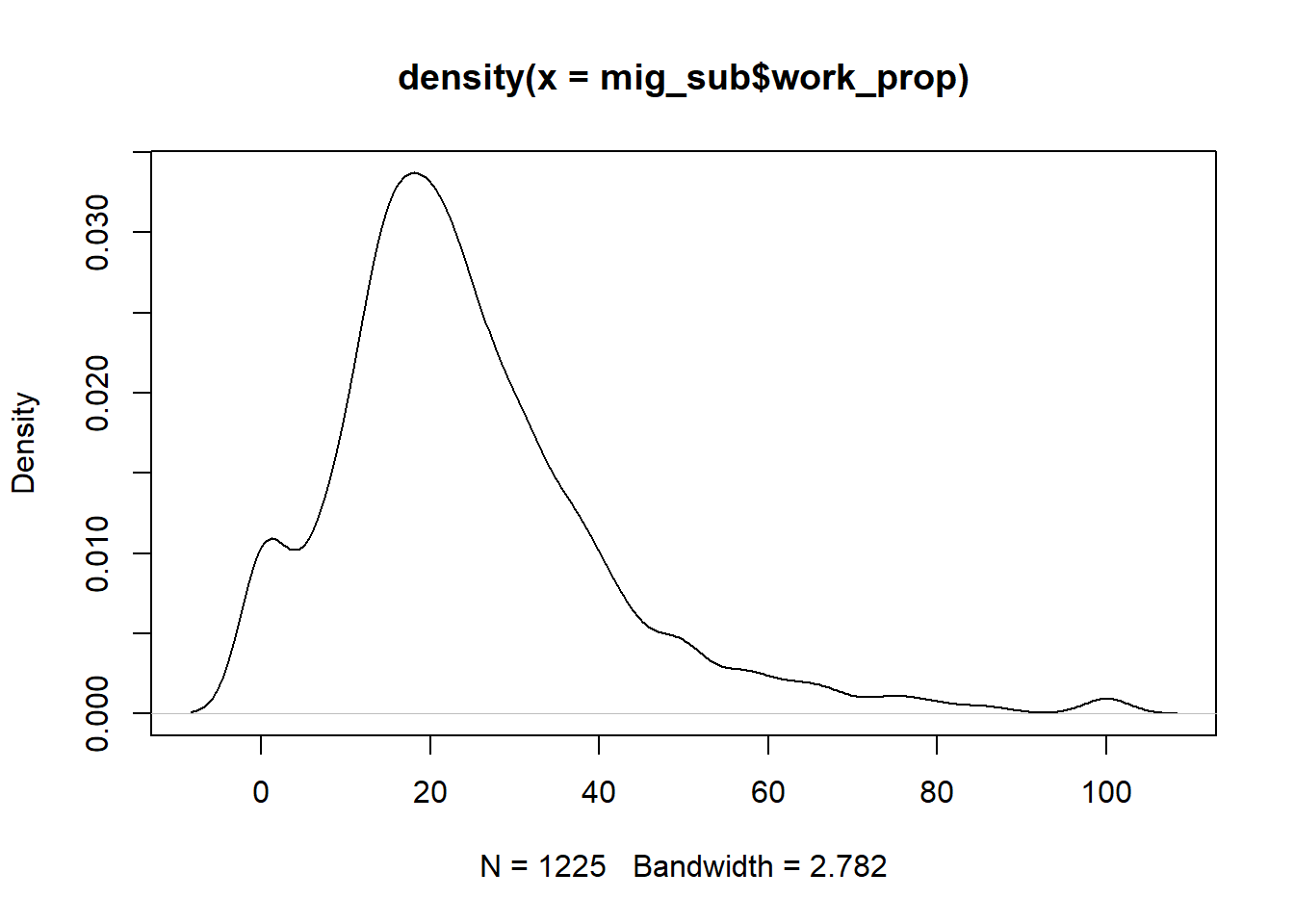

Code

plot(density(mig_sub$educ_prop))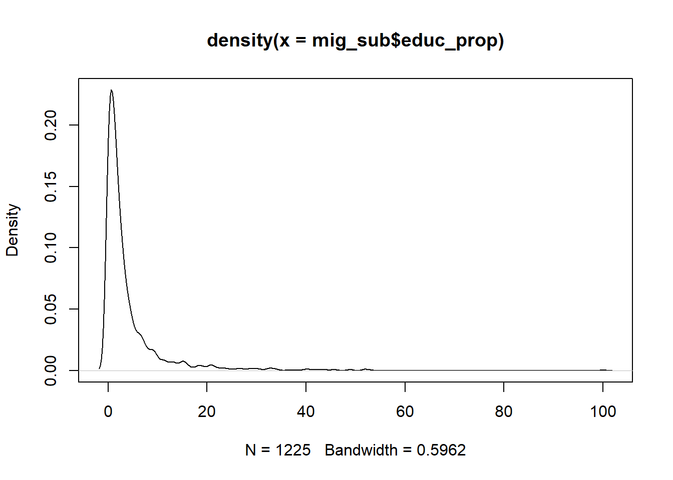

Code

plot(density(mig_sub$mar_prop))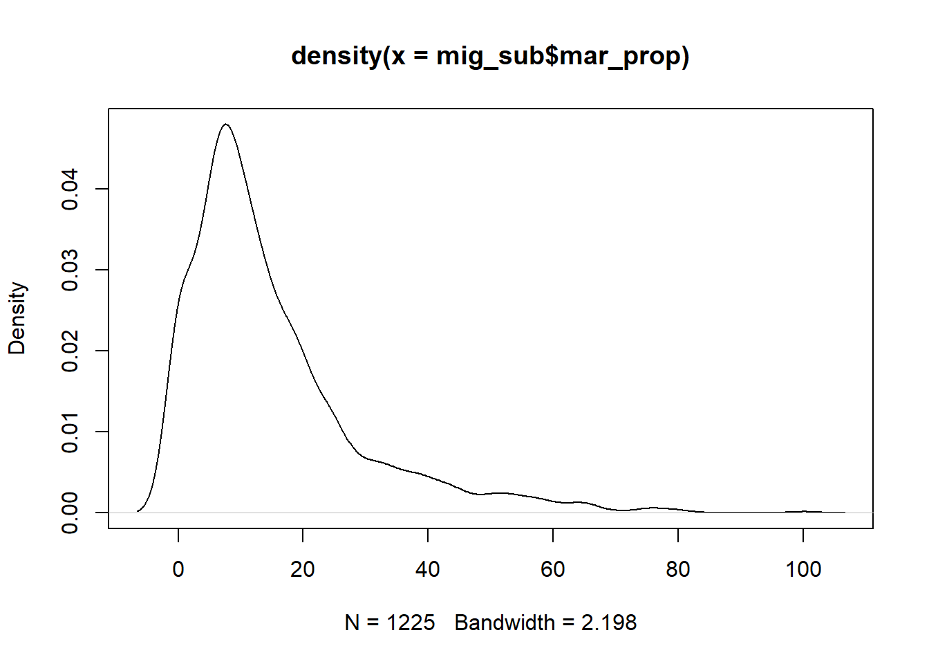

Code

cor(mig_sub$mar_prop, mig_sub$work_prop)

[1] -0.2868978

Code

cor(mig_sub$educ_prop, mig_sub$work_prop)

[1] -0.07564778

Code

cor(mig_sub$educ_prop, mig_sub$mar_prop)

[1] -0.1854825

Code

lm(mig_sub$work_prop~mig_sub$mar_prop)


Call:
lm(formula = mig_sub$work_prop ~ mig_sub$mar_prop)

Coefficients:
     (Intercept)  mig_sub$mar_prop  
         29.3850           -0.3361

Code

reg1<-lm(mig_sub$work_prop~mig_sub$mar_prop)
summary(reg1)


Call:
lm(formula = mig_sub$work_prop ~ mig_sub$mar_prop)

Residuals:
    Min      1Q  Median      3Q     Max 
-29.385  -8.584  -1.435   6.655  70.615 

Coefficients:
                 Estimate Std. Error t value Pr(>|t|)    
(Intercept)      29.38497    0.65622   44.78   <2e-16 ***
mig_sub$mar_prop -0.33612    0.03209  -10.47   <2e-16 ***
---
Signif. codes:  0 '***' 0.001 '**' 0.01 '*' 0.05 '.' 0.1 ' ' 1

Residual standard error: 15.75 on 1223 degrees of freedom
Multiple R-squared:  0.08231,   Adjusted R-squared:  0.08156 
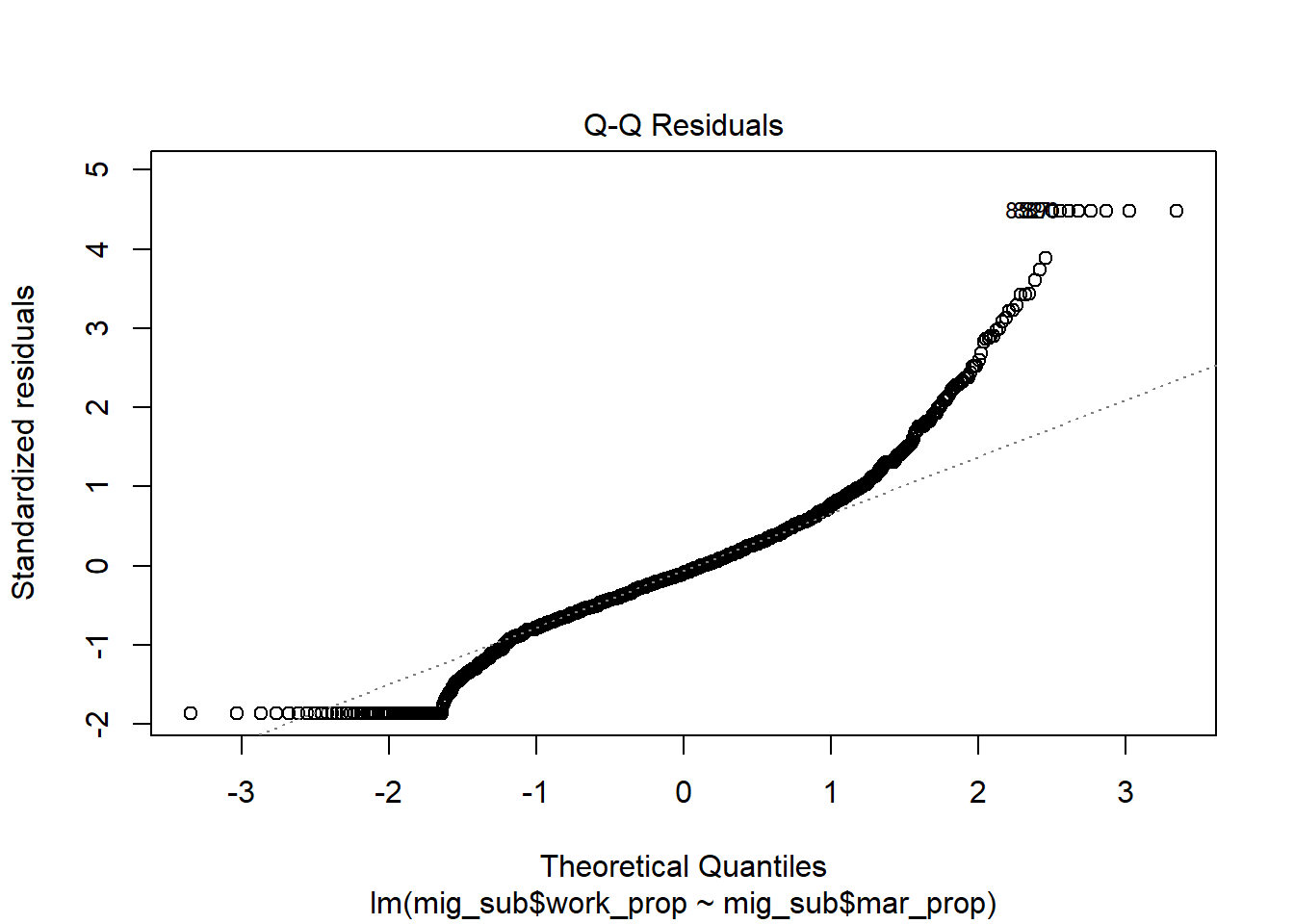
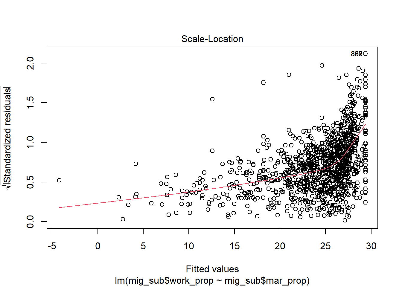
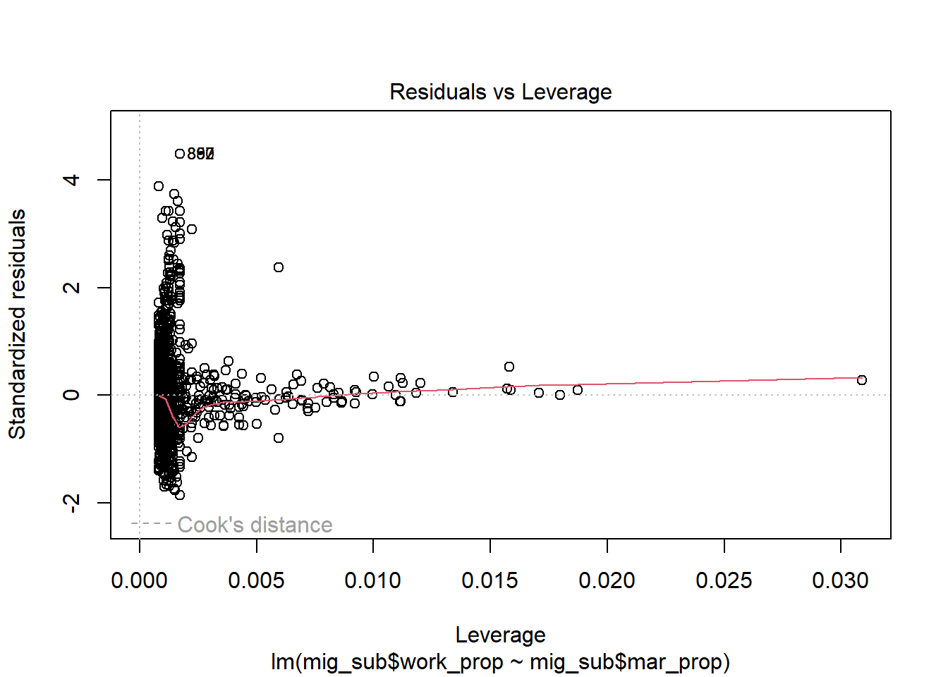
F-statistic: 109.7 on 1 and 1223 DF,  p-value: < 2.2e-16

Code

 plot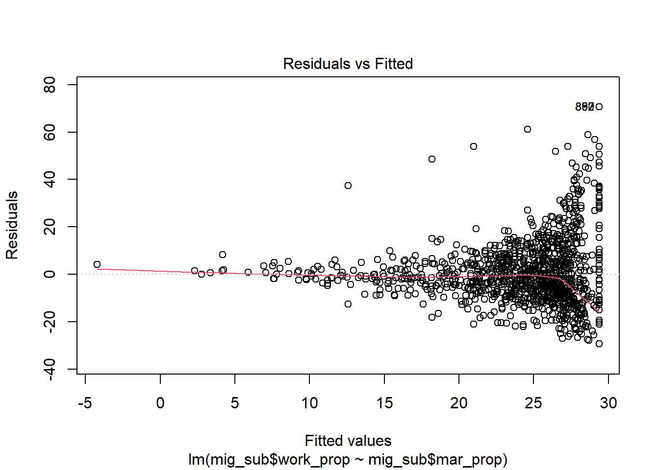(reg1)

Selecting a threshold

Using the data as it currently is would make the network too dense. There is movement between almost every state and some of these movements are irrelevant because the proportion is smaller than 1%. Hence, I looked into the distributions of the proportions of people who moved for work and marriage, in order to decide a threshold.

Using work as the weight

Code

mig_network<-mig_sub%>%
  relocate(work_prop,.before=tot_t)%>%
  rename(from=last_res,to=area,weight=work_prop)
mig_network<-mig_network[1:3]

hist(mig_network$weight)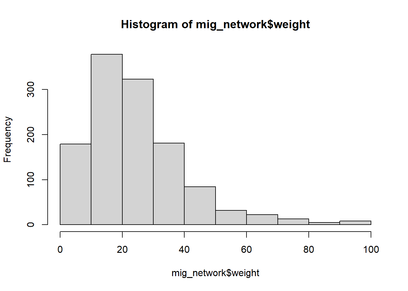

Code

quantile(mig_network$weight)

    0%    25%    50%    75%   100% 
  0.00  14.29  21.43  31.46 100.00

Using marriage as the weight

Code

mig_mar<-mig_sub%>%
  relocate(mar_prop,.before=tot_t)%>%
  rename(from=last_res,to=area,weight=mar_prop)
mig_mar<-mig_mar[1:3]

hist(mig_mar$weight)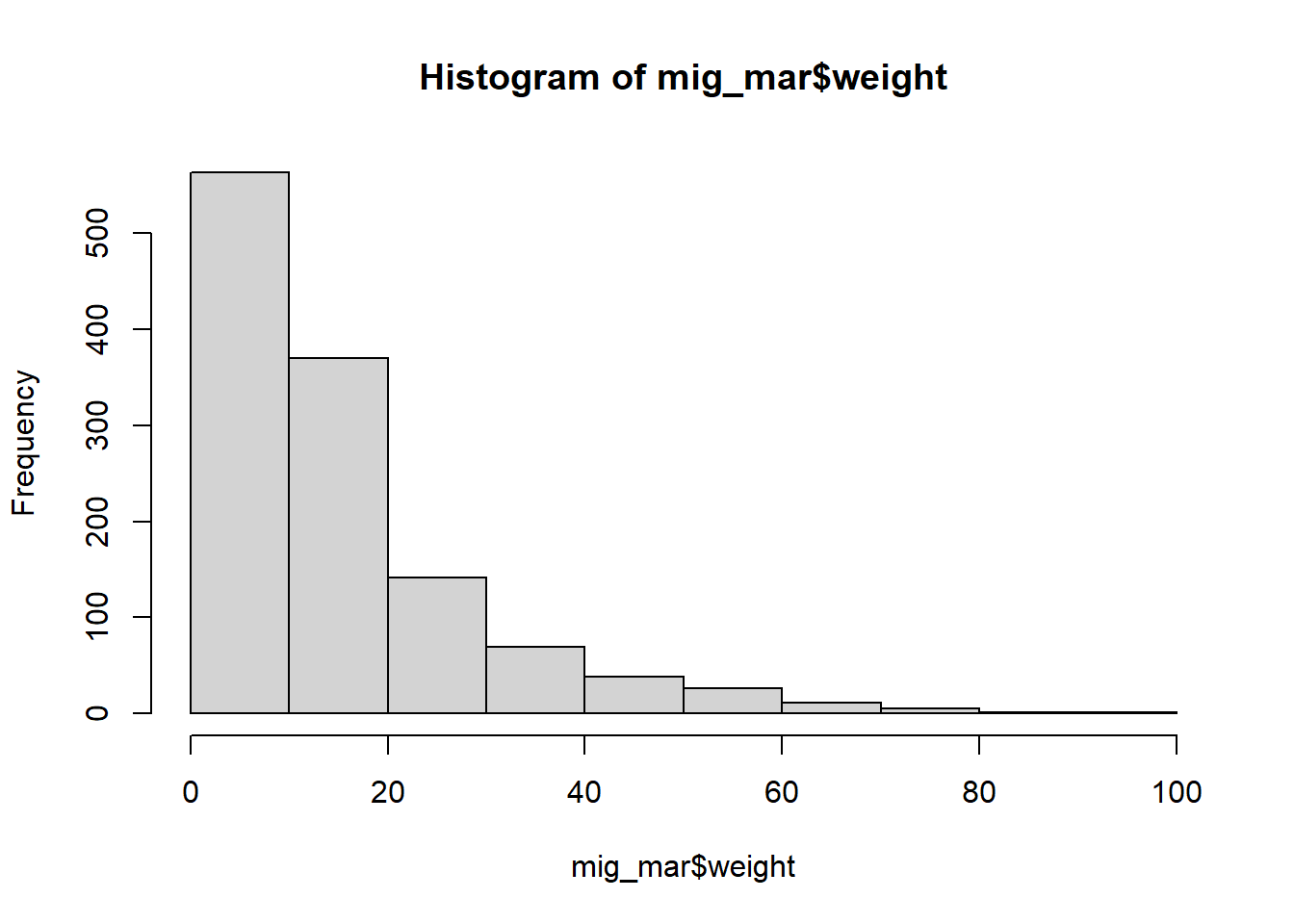

Code

quantile(mig_mar$weight)

    0%    25%    50%    75%   100% 
  0.00   5.88  10.91  19.45 100.00

Threshold

After observing the distribution of the proportions of the reasons along with the quantiles, I decided to keep a threshold of 20%, this would roughly cover about half of the total observations for people who moved for work and the last quantile of the people who moved due to marriage.

Creating the networks

Network based on work

Code

mig_net_threshold<- mig_network%>% 
 filter(weight>=20)
dim(mig_network)

[1] 1225    3

Code

dim(mig_net_threshold)

[1] 676   3

Code

mig_work_ig<-igraph::graph_from_data_frame(mig_net_threshold,directed=TRUE)
mig_work_stat<-network(mig_net_threshold,matrix.type="edgelist")

Network based on marriage

Code

mig_mar_threshold <- mig_mar%>%
  filter(weight>=20)
dim(mig_mar_threshold)

[1] 294   3

Code

mig_mar_ig<-igraph::graph_from_data_frame(mig_mar_threshold,directed=TRUE)
mig_mar_stat<-network(mig_mar_threshold,matrix.type="edgelist")

Descriptives of all the networks

I kept both the descriptives from statnet and igraph because in a previous challenge, I found inconsistencies in the number of edges and other details and wanted to make sure that the same issue is not occurring here.

Description for migration for work

Code

print(mig_work_stat)

 Network attributes:
  vertices = 35 
  directed = TRUE 
  hyper = FALSE 
  loops = FALSE 
  multiple = FALSE 
  bipartite = FALSE 
  total edges= 676 
    missing edges= 0 
    non-missing edges= 676 

 Vertex attribute names: 
    vertex.names 

 Edge attribute names: 
    weight

Code

vcount(mig_work_ig)

[1] 35

Code

ecount(mig_work_ig)

[1] 676

Code

is_bipartite(mig_work_ig)

[1] FALSE

Code

is_directed(mig_work_ig)

[1] TRUE

Code

is_weighted(mig_work_ig)

[1] TRUE

Description for migration due to marriage

Code

print(mig_mar_stat)

 Network attributes:
  vertices = 35 
  directed = TRUE 
  hyper = FALSE 
  loops = FALSE 
  multiple = FALSE 
  bipartite = FALSE 
  total edges= 294 
    missing edges= 0 
    non-missing edges= 294 

 Vertex attribute names: 
    vertex.names 

 Edge attribute names: 
    weight

Code

vcount(mig_mar_ig)

[1] 35

Code

ecount(mig_mar_ig)

[1] 294

Code

is_bipartite(mig_mar_ig)

[1] FALSE

Code

is_directed(mig_mar_ig)

[1] TRUE

Code

is_weighted(mig_mar_ig)

[1] TRUE

Components

There is 1 component for the migrant network pertaining to movement for work as well as for the network pertaining to movement for marriage which means that both are connected graphs.

Code

names(igraph::components(mig_work_ig))

[1] "membership" "csize"      "no"

Code

#igraph::components(mig.ig)$membership
igraph::components(mig_work_ig)$no

[1] 1

Code

igraph::components(mig_work_ig)$csize

[1] 35

Code

names(igraph::components(mig_mar_ig))

[1] "membership" "csize"      "no"

Code

#igraph::components(mig.ig)$membership
igraph::components(mig_mar_ig)$no

[1] 1

Code

igraph::components(mig_mar_ig)$csize

[1] 35

Density

Since a threshold was set after checking the quantiles, the density was manually created. However, these figures do show that for the same threshold, the migrant network for movement for work is more dense than the migrant network for movement for marriage. This illustrates that more people tend to move for economic opportunities in comparison to marriage.

Code

graph.density(mig_work_ig,loops=FALSE)

[1] 0.5680672

Code

graph.density(mig_mar_ig,loops=FALSE)

[1] 0.2470588

Plotting the networks

The plots of the networks visually demonstrate the density.

Code

# switch to statnet object to plot
ggnet2(mig_work_stat,label=TRUE,label.size=2.5, arrow.size = 5, arrow.gap = 0.03,color = rep("#48bfe3", 35))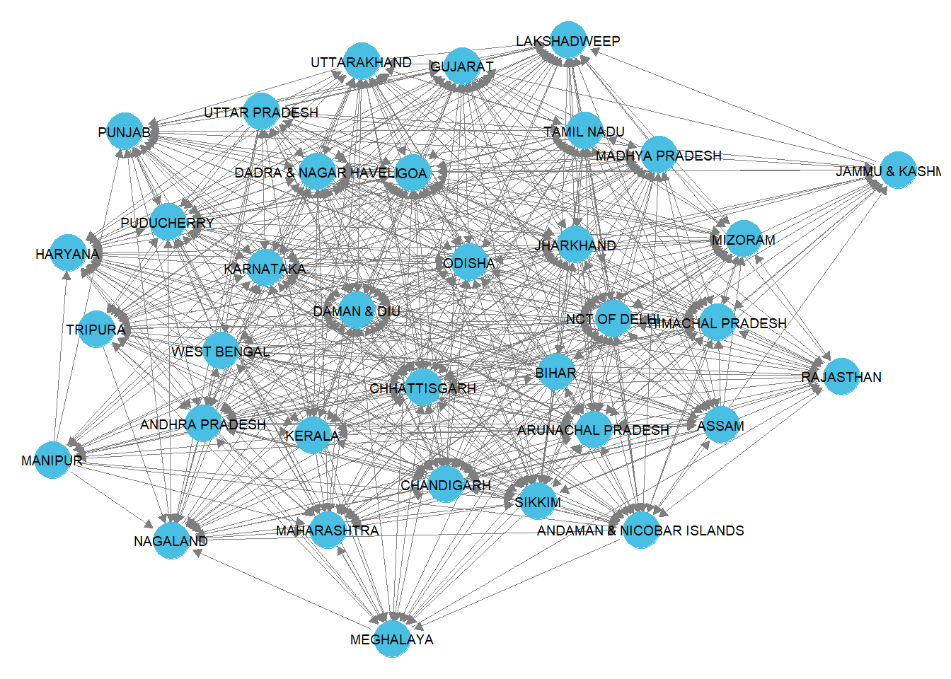

Code

#save a ggnet layout that you like

Code

# switch to statnet object to plot
ggnet2(mig_mar_stat,label=TRUE,label.size=2.5, arrow.size = 5, arrow.gap = 0.03,color = rep("#48bfe3", 35))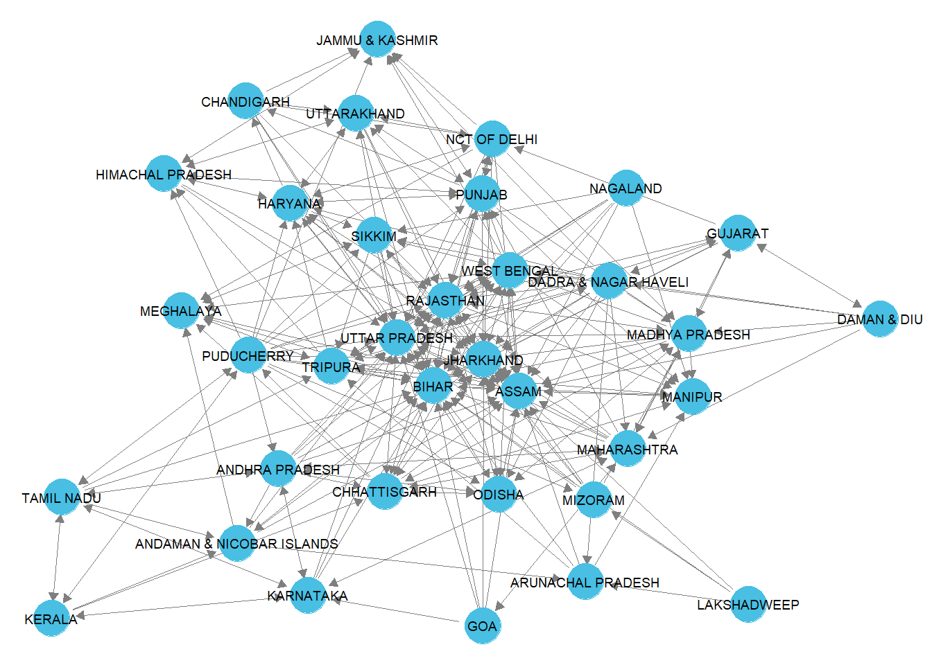

Code

#save a ggnet layout that you like

Creating the dataframes to store different measures of networks

Code

Set <- c("#7400b8","#8400d2","#5e60ce", "#5390d9","#689dde", "#48bfe3", "#64dfdf", "#72efdd", "#89f2e3","#80ffdb")

Code

nodes_w<-data.frame(name = V(mig_work_ig)$name,
    all.degree = igraph::degree(mig_work_ig, mode = 'all'), 
    out.degree = igraph::degree(mig_work_ig, mode = 'out'),
    in.degree = igraph::degree(mig_work_ig, mode = 'in'), 
    strength_all=igraph::strength(mig_work_ig),
    strength_in=igraph::strength(mig_work_ig,mode="in"),
    strength_out=igraph::strength(mig_work_ig,mode="out"),
    cons=igraph::constraint(mig_work_ig),
    eigen=igraph:: evcent(mig_work_ig)$vector)
nodes_w$transitivity <- transitivity(mig_work_ig, type = 'local')
nodes_w$weighted.transitivity <-  transitivity(mig_work_ig, type = 'weighted')
gtrans(mig_work_stat)

[1] 0.7104843

Code

summary(nodes_w)

     name             all.degree      out.degree      in.degree    
 Length:35          Min.   :19.00   Min.   : 6.00   Min.   : 4.00  
 Class :character   1st Qu.:34.00   1st Qu.:15.00   1st Qu.:14.00  
 Mode  :character   Median :38.00   Median :20.00   Median :19.00  
                    Mean   :38.63   Mean   :19.31   Mean   :19.31  
                    3rd Qu.:44.00   3rd Qu.:24.00   3rd Qu.:25.50  
                    Max.   :53.00   Max.   :32.00   Max.   :32.00  
  strength_all     strength_in      strength_out         cons       
 Min.   : 551.9   Min.   : 115.7   Min.   : 195.5   Min.   :0.1163  
 1st Qu.:1136.4   1st Qu.: 435.0   1st Qu.: 454.6   1st Qu.:0.1232  
 Median :1295.2   Median : 556.1   Median : 594.1   Median :0.1248  
 Mean   :1338.5   Mean   : 669.2   Mean   : 669.2   Mean   :0.1270  
 3rd Qu.:1587.9   3rd Qu.: 840.1   3rd Qu.: 838.9   3rd Qu.:0.1290  
 Max.   :2289.3   Max.   :1704.7   Max.   :1385.0   Max.   :0.1495  
     eigen         transitivity    weighted.transitivity
 Min.   :0.2803   Min.   :0.8044   Min.   :0.6376       
 1st Qu.:0.5246   1st Qu.:0.8312   1st Qu.:0.8294       
 Median :0.6119   Median :0.8519   Median :0.8869       
 Mean   :0.6138   Mean   :0.8546   Mean   :0.8977       
 3rd Qu.:0.7122   3rd Qu.:0.8741   3rd Qu.:0.9883       
 Max.   :1.0000   Max.   :0.9265   Max.   :1.1905

Code

nodes_m<-data.frame(name = V(mig_mar_ig)$name,
    all.degree = igraph::degree(mig_mar_ig, mode = 'all'), 
    out.degree = igraph::degree(mig_mar_ig, mode = 'out'),
    in.degree = igraph::degree(mig_mar_ig, mode = 'in'), 
    strength_all=igraph::strength(mig_mar_ig),
    strength_in=igraph::strength(mig_mar_ig,mode="in"),
    strength_out=igraph::strength(mig_mar_ig,mode="out"),
    cons=igraph::constraint(mig_mar_ig),
    eigen=igraph:: evcent(mig_mar_ig)$vector)
#Global
transitivity(mig_mar_ig, type="global")

[1] 0.5459427

Code

##Average local clustering coefficient
transitivity(mig_mar_ig, type="average")

[1] 0.6267173

Code

nodes_m$transitivity <- transitivity(mig_mar_ig, type = 'local')
nodes_m$weighted.transitivity <-  transitivity(mig_mar_ig, type = 'weighted')
gtrans(mig_mar_stat)

[1] 0.5551987

Code

summary(nodes_m)

     name             all.degree     out.degree     in.degree   
 Length:35          Min.   : 4.0   Min.   : 2.0   Min.   : 0.0  
 Class :character   1st Qu.: 9.0   1st Qu.: 6.0   1st Qu.: 3.0  
 Mode  :character   Median :14.0   Median : 8.0   Median : 7.0  
                    Mean   :16.8   Mean   : 8.4   Mean   : 8.4  
                    3rd Qu.:21.0   3rd Qu.:11.0   3rd Qu.: 9.5  
                    Max.   :36.0   Max.   :16.0   Max.   :30.0  
  strength_all     strength_in       strength_out         cons       
 Min.   : 130.7   Min.   :   0.00   Min.   : 71.72   Min.   :0.1452  
 1st Qu.: 323.5   1st Qu.:  98.95   1st Qu.:167.34   1st Qu.:0.1917  
 Median : 463.9   Median : 200.00   Median :247.94   Median :0.2197  
 Mean   : 584.7   Mean   : 292.35   Mean   :292.35   Mean   :0.2298  
 3rd Qu.: 799.0   3rd Qu.: 337.69   3rd Qu.:392.85   3rd Qu.:0.2642  
 Max.   :1534.2   Max.   :1352.18   Max.   :742.49   Max.   :0.3482  
     eigen          transitivity    weighted.transitivity
 Min.   :0.06377   Min.   :0.3862   Min.   :0.3933       
 1st Qu.:0.18972   1st Qu.:0.5303   1st Qu.:0.5362       
 Median :0.33821   Median :0.6167   Median :0.6468       
 Mean   :0.41009   Mean   :0.6267   Mean   :0.6914       
 3rd Qu.:0.58714   3rd Qu.:0.7022   3rd Qu.:0.7736       
 Max.   :1.00000   Max.   :0.9091   Max.   :1.3039

Transitivity

In the migration network weighted for movement due to work, the transitivity values for the global and average clustering coefficients are both roughly 0.85. This depicts that every state is connected to almost every other remaining state. In other words, migration occurs between almost all states. However, the proportion of migrants for each connection may not be a significant amount. This is explored by using strength as a network measure.

In the migration network weighted for movement due to marriage, the transitivity is lower, with a global clustering coefficient of roughly 0.55 and local clustering coefficient of roughly 0.63. This demonstrates that there are densely interconnected subgroups. It also shows that when it comes to migration for marriage, people are more selective.

In India, arranged marriages are common and marriages within the same caste are preferred (Sahgal et al., 2021). The caste system is a social stratification system; one is born into a fixed social group referred to as their caste (“Systems of Social Stratification”, n.d.). While people of the same caste can reside in multiple states, perhaps the cultural differences between states result in people being more selective about marriage.

Many states have their own languages, distinct food, festivals, etc. Often the language or food habits may be similar for neighbouring states. Therefore, it may be the case that the subgroups are formed based on neighbouring states since one would prefer to marry someone who is culturally similar. Whether the subgroups are based on states that share boundaries or in a particular region can be explored through clustering.

Code

#Global
transitivity(mig_work_ig, type="global")

[1] 0.8484054

Code

##Average local clustering coefficient
transitivity(mig_work_ig, type="average")

[1] 0.8546428

Code

melt(nodes_w) %>% filter(variable == 'transitivity' | variable == 'weighted.transitivity') %>% 
  ggplot(aes(x = value, fill = variable, color = variable)) + geom_density(alpha = 0.2) +
  ggtitle('Transitivity Distribution, Local and Weighted for Migration due to Work')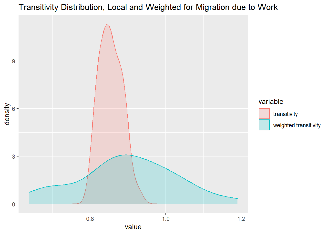

Code

#Global
transitivity(mig_mar_ig, type="global")

[1] 0.5459427

Code

##Average local clustering coefficient
transitivity(mig_mar_ig, type="average")

[1] 0.6267173

Code

melt(nodes_m) %>% filter(variable == 'transitivity' | variable == 'weighted.transitivity') %>% 
  ggplot(aes(x = value, fill = variable, color = variable)) + geom_density(alpha = 0.2) +
  ggtitle('Transitivity Distribution, Local and Weighted for Migration due to Marriage')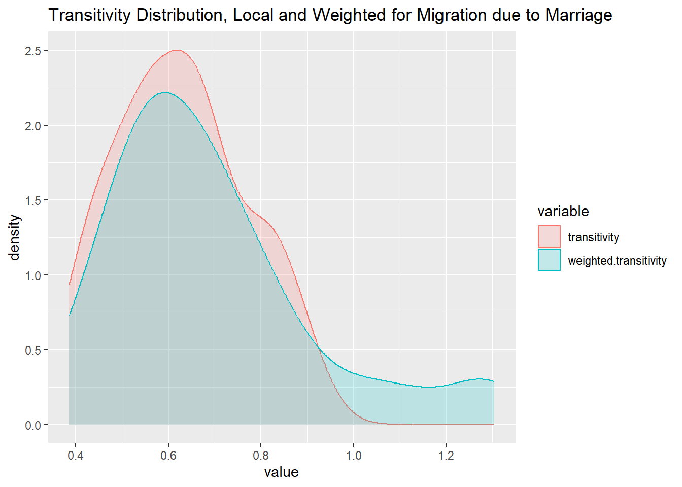

Degree overview

The measures of degree represent how certain states have multiple connections, however, since there are weights this might not be the most accurate depiction. This is because some states could have many ties with other states but the proportion of people who are moving could be low. Therefore, I looked into the strength measure which takes the weights into account.

Code

nodes_w%>%select("name","all.degree","in.degree","out.degree")%>%arrange(desc(all.degree))

                                               name all.degree in.degree
CHHATTISGARH                           CHHATTISGARH         53        26
NCT OF DELHI                           NCT OF DELHI         52        32
JHARKHAND                                 JHARKHAND         50        20
GOA                                             GOA         50        29
DAMAN & DIU                             DAMAN & DIU         49        32
ODISHA                                       ODISHA         48        17
SIKKIM                                       SIKKIM         45        24
KARNATAKA                                 KARNATAKA         45        25
ANDHRA PRADESH                       ANDHRA PRADESH         44        19
KERALA                                       KERALA         44        13
CHANDIGARH                               CHANDIGARH         44        28
ARUNACHAL PRADESH                 ARUNACHAL PRADESH         43        29
TAMIL NADU                               TAMIL NADU         42        15
MADHYA PRADESH                       MADHYA PRADESH         40        17
UTTARAKHAND                             UTTARAKHAND         40        17
GUJARAT                                     GUJARAT         40        23
TRIPURA                                     TRIPURA         39        17
DADRA & NAGAR HAVELI           DADRA & NAGAR HAVELI         38        31
PUDUCHERRY                               PUDUCHERRY         38        18
HIMACHAL PRADESH                   HIMACHAL PRADESH         37        25
BIHAR                                         BIHAR         36         4
MIZORAM                                     MIZORAM         36        21
MAHARASHTRA                             MAHARASHTRA         36        26
UTTAR PRADESH                         UTTAR PRADESH         35         7
ANDAMAN & NICOBAR ISLANDS ANDAMAN & NICOBAR ISLANDS         35        23
ASSAM                                         ASSAM         34        11
NAGALAND                                   NAGALAND         34        18
WEST BENGAL                             WEST BENGAL         33         7
HARYANA                                     HARYANA         33        21
LAKSHADWEEP                             LAKSHADWEEP         33        27
PUNJAB                                       PUNJAB         30        15
RAJASTHAN                                 RAJASTHAN         28        11
MEGHALAYA                                 MEGHALAYA         27        12
MANIPUR                                     MANIPUR         22         6
JAMMU & KASHMIR                     JAMMU & KASHMIR         19        10
                          out.degree
CHHATTISGARH                      27
NCT OF DELHI                      20
JHARKHAND                         30
GOA                               21
DAMAN & DIU                       17
ODISHA                            31
SIKKIM                            21
KARNATAKA                         20
ANDHRA PRADESH                    25
KERALA                            31
CHANDIGARH                        16
ARUNACHAL PRADESH                 14
TAMIL NADU                        27
MADHYA PRADESH                    23
UTTARAKHAND                       23
GUJARAT                           17
TRIPURA                           22
DADRA & NAGAR HAVELI               7
PUDUCHERRY                        20
HIMACHAL PRADESH                  12
BIHAR                             32
MIZORAM                           15
MAHARASHTRA                       10
UTTAR PRADESH                     28
ANDAMAN & NICOBAR ISLANDS         12
ASSAM                             23
NAGALAND                          16
WEST BENGAL                       26
HARYANA                           12
LAKSHADWEEP                        6
PUNJAB                            15
RAJASTHAN                         17
MEGHALAYA                         15
MANIPUR                           16
JAMMU & KASHMIR                    9

Code

nodes_m%>%select("name","all.degree","in.degree","out.degree")%>%arrange(desc(all.degree))

                                               name all.degree in.degree
BIHAR                                         BIHAR         36        30
ASSAM                                         ASSAM         35        25
UTTAR PRADESH                         UTTAR PRADESH         35        26
RAJASTHAN                                 RAJASTHAN         32        20
JHARKHAND                                 JHARKHAND         32        24
WEST BENGAL                             WEST BENGAL         28        14
PUNJAB                                       PUNJAB         23        10
MADHYA PRADESH                       MADHYA PRADESH         22        11
HARYANA                                     HARYANA         21        10
CHHATTISGARH                           CHHATTISGARH         21         9
MAHARASHTRA                             MAHARASHTRA         20         8
PUDUCHERRY                               PUDUCHERRY         19         3
TRIPURA                                     TRIPURA         19         9
DADRA & NAGAR HAVELI           DADRA & NAGAR HAVELI         18         3
ODISHA                                       ODISHA         17         8
ANDHRA PRADESH                       ANDHRA PRADESH         17         5
NCT OF DELHI                           NCT OF DELHI         16         5
UTTARAKHAND                             UTTARAKHAND         14         7
GUJARAT                                     GUJARAT         14         5
SIKKIM                                       SIKKIM         14         7
MEGHALAYA                                 MEGHALAYA         13         8
HIMACHAL PRADESH                   HIMACHAL PRADESH         12         6
KARNATAKA                                 KARNATAKA         12         5
MANIPUR                                     MANIPUR         12         9
TAMIL NADU                               TAMIL NADU         11         4
JAMMU & KASHMIR                     JAMMU & KASHMIR          9         7
ANDAMAN & NICOBAR ISLANDS ANDAMAN & NICOBAR ISLANDS          9         4
CHANDIGARH                               CHANDIGARH          8         2
NAGALAND                                   NAGALAND          8         0
MIZORAM                                     MIZORAM          8         2
KERALA                                       KERALA          8         3
GOA                                             GOA          7         1
ARUNACHAL PRADESH                 ARUNACHAL PRADESH          7         3
DAMAN & DIU                             DAMAN & DIU          7         1
LAKSHADWEEP                             LAKSHADWEEP          4         0
                          out.degree
BIHAR                              6
ASSAM                             10
UTTAR PRADESH                      9
RAJASTHAN                         12
JHARKHAND                          8
WEST BENGAL                       14
PUNJAB                            13
MADHYA PRADESH                    11
HARYANA                           11
CHHATTISGARH                      12
MAHARASHTRA                       12
PUDUCHERRY                        16
TRIPURA                           10
DADRA & NAGAR HAVELI              15
ODISHA                             9
ANDHRA PRADESH                    12
NCT OF DELHI                      11
UTTARAKHAND                        7
GUJARAT                            9
SIKKIM                             7
MEGHALAYA                          5
HIMACHAL PRADESH                   6
KARNATAKA                          7
MANIPUR                            3
TAMIL NADU                         7
JAMMU & KASHMIR                    2
ANDAMAN & NICOBAR ISLANDS          5
CHANDIGARH                         6
NAGALAND                           8
MIZORAM                            6
KERALA                             5
GOA                                6
ARUNACHAL PRADESH                  4
DAMAN & DIU                        6
LAKSHADWEEP                        4

Strength

Code

nodes_w %>% melt %>%filter(variable=='strength_all'|variable=='strength_in'|variable=='strength_out')%>%
  ggplot(aes(x = value, fill = variable, color = variable)) + geom_density(alpha = .2, bw = 5) +
  ggtitle('Strength Distribution')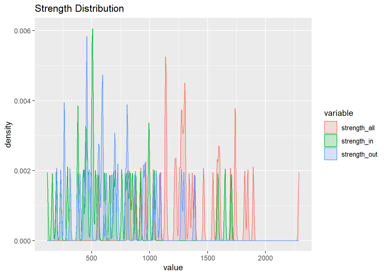

Code

nodes_m %>% melt %>%filter(variable=='strength_all'|variable=='strength_in'|variable=='strength_out')%>%
  ggplot(aes(x = value, fill = variable, color = variable)) + geom_density(alpha = .2, bw = 5) +
  ggtitle('Strength Distribution')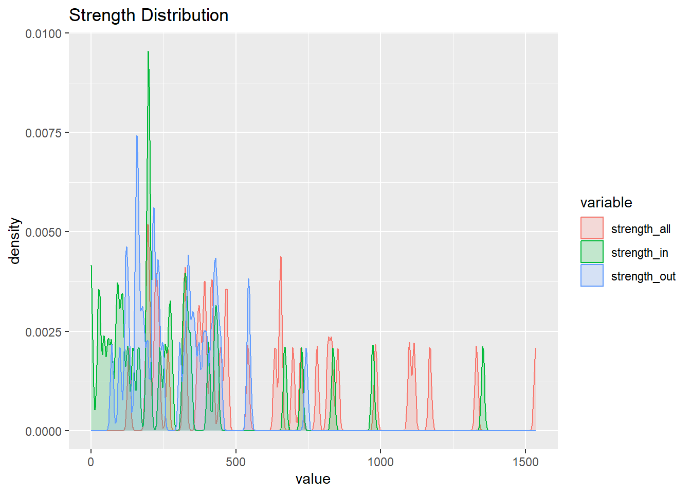

Strength- Out

For the migrants moving out for work, it is interesting to see that the top 3 states are neighbouring states. West Bengal, Chhattisgarh and Uttar Pradesh also share borders with the top 3 states. So there is majorly out migration from work occurring from the Eastern part and a bit of the Northern part of India . This suggests that these regions may not have as many economic opportunities or chances for growth.

For the movement due to marriage, 2 of the top 3 places (Dadra & Nagar Haveli and Puducherry) are union territories which have a smaller population in comparison to other states. Additionally, a prominent region of out migration for marriage can be observed from the North western region of India (Punjab, Rajasthan and Haryana).

Code

out_w<-nodes_w %>% arrange(desc(strength_out))%>%slice(1:10)
ggplot(out_w, aes(fill=name,x=reorder(name,strength_out),y=strength_out))+ 
  geom_bar(stat = "identity")+
  scale_fill_manual(values=Set,guide="none")+
  coord_flip()+
  geom_text(aes(label=round(strength_out,digits=2)),position=position_stack(vjust=0.5))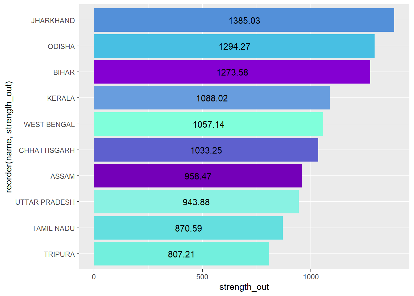

Code

out_m<-nodes_m%>% arrange(desc(strength_out))%>%slice(1:10)
ggplot(out_m, aes(fill=name,x=reorder(name,strength_out),y=strength_out))+ 
  geom_bar(stat = "identity")+
  scale_fill_manual(values=Set,guide="none")+
  coord_flip()+
  geom_text(aes(label=round(strength_out,digits=2)),position=position_stack(vjust=0.5))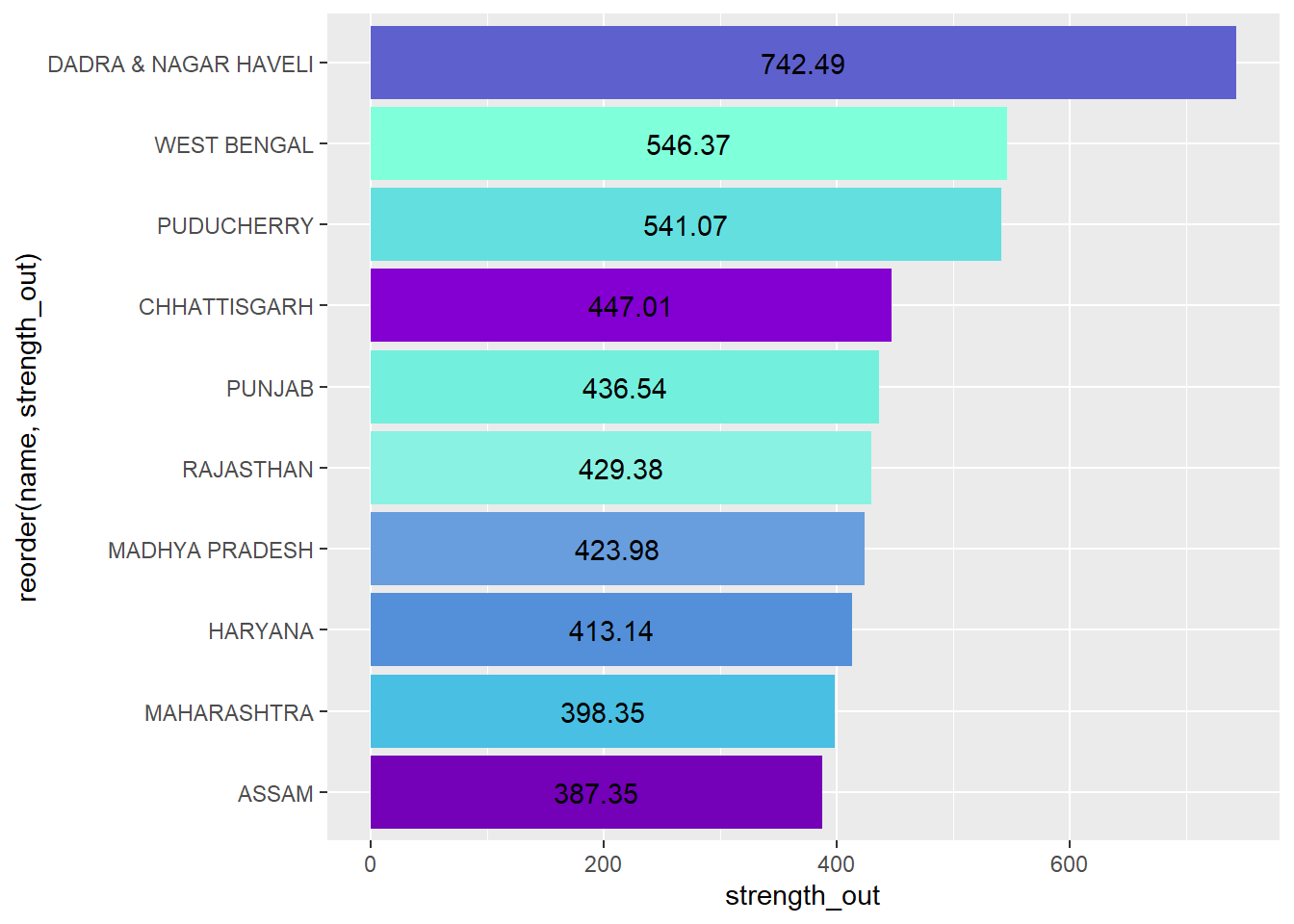

Strength- In

For the migrants moving to places for work, the top 3 receiving states are union territories. There is no prominent region which has in-migration, the states in the graph are from various parts of India.

For the receiving states of migrants who move for marriage, interestingly, the top 3 states are the same states that fell among the top 10 in those who moved out for work. There is also a significant overlap in the states that sent out migrants due to marriage and also receive migrants due to marriage- Assam, Rajasthan, West Bengal and Haryana. It may be the case that many people move between Haryana and Rajasthan since they are neighbouring states. Similary, since one of the neighbouring states to Assam is West Bengal, more people between the two due to marriage.

Code

in_w<-nodes_w %>% arrange(desc(strength_in))%>%slice(1:10)
ggplot(in_w, aes(fill=name,x=reorder(name,strength_in),y=strength_in))+ 
  geom_bar(stat = "identity")+
  scale_fill_manual(values=Set,guide="none")+
  coord_flip()+
  geom_text(aes(label=round(strength_in,digits=2)),position=position_stack(vjust=0.5))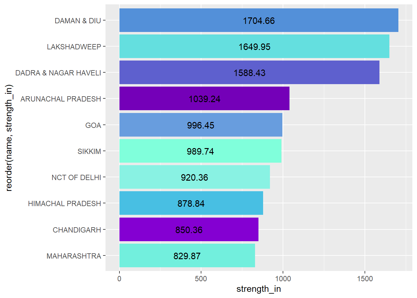

Code

in_m<-nodes_m %>% arrange(desc(strength_in))%>%slice(1:10)
ggplot(in_m, aes(fill=name,x=reorder(name,strength_in),y=strength_in))+ 
  geom_bar(stat = "identity")+
  scale_fill_manual(values=Set,guide="none")+
  coord_flip()+
  geom_text(aes(label=round(strength_in,digits=2)),position=position_stack(vjust=0.5))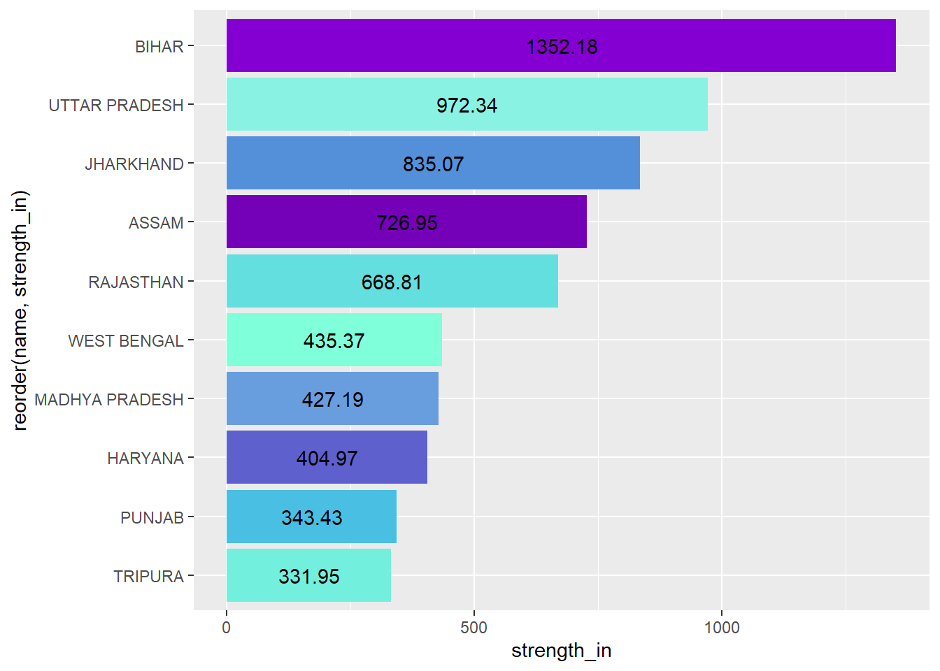

Eigenvector centrality, Constraint, Diameter

The following tables show the eigenvector centralities and constraints for the nodes of the 2 networks. The diameters for the two networks has also been provided.

However, since the data did not record dynamic migration, that is the same person moving to more than one state in the time frame studied, the indirect connections between each node are not significant/ they do not represent movement. Since the measures in this section depict how nodes are connected to nodes that are central, information flow between nodes that are indirectly connected and the distance between one node to the other, they do not give interpretable information for the case of the migrant networks in this study.

Code

nodes_w %>% select(name,eigen)%>%arrange(desc(eigen))

                                               name     eigen
DAMAN & DIU                             DAMAN & DIU 1.0000000
LAKSHADWEEP                             LAKSHADWEEP 0.8448656
JHARKHAND                                 JHARKHAND 0.8283580
DADRA & NAGAR HAVELI           DADRA & NAGAR HAVELI 0.8082074
ODISHA                                       ODISHA 0.7657562
CHHATTISGARH                           CHHATTISGARH 0.7586060
GOA                                             GOA 0.7465529
ARUNACHAL PRADESH                 ARUNACHAL PRADESH 0.7272429
KERALA                                       KERALA 0.7155870
NCT OF DELHI                           NCT OF DELHI 0.7088015
SIKKIM                                       SIKKIM 0.7012270
MIZORAM                                     MIZORAM 0.6656215
TRIPURA                                     TRIPURA 0.6369395
BIHAR                                         BIHAR 0.6259032
KARNATAKA                                 KARNATAKA 0.6204448
UTTARAKHAND                             UTTARAKHAND 0.6183229
ASSAM                                         ASSAM 0.6127363
TAMIL NADU                               TAMIL NADU 0.6118898
CHANDIGARH                               CHANDIGARH 0.6058887
PUDUCHERRY                               PUDUCHERRY 0.5941980
HIMACHAL PRADESH                   HIMACHAL PRADESH 0.5901149
MADHYA PRADESH                       MADHYA PRADESH 0.5864338
ANDHRA PRADESH                       ANDHRA PRADESH 0.5736233
WEST BENGAL                             WEST BENGAL 0.5645886
UTTAR PRADESH                         UTTAR PRADESH 0.5415897
GUJARAT                                     GUJARAT 0.5324478
ANDAMAN & NICOBAR ISLANDS ANDAMAN & NICOBAR ISLANDS 0.5166731
MAHARASHTRA                             MAHARASHTRA 0.4919679
NAGALAND                                   NAGALAND 0.4818445
HARYANA                                     HARYANA 0.4627093
PUNJAB                                       PUNJAB 0.4485455
RAJASTHAN                                 RAJASTHAN 0.4298923
MANIPUR                                     MANIPUR 0.4084978
MEGHALAYA                                 MEGHALAYA 0.3754753
JAMMU & KASHMIR                     JAMMU & KASHMIR 0.2803492

Code

nodes_m %>% select(name,eigen)%>%arrange(desc(eigen))

                                               name      eigen
BIHAR                                         BIHAR 1.00000000
UTTAR PRADESH                         UTTAR PRADESH 0.96855016
JHARKHAND                                 JHARKHAND 0.87264309
RAJASTHAN                                 RAJASTHAN 0.79904410
WEST BENGAL                             WEST BENGAL 0.75755352
ASSAM                                         ASSAM 0.74267866
MADHYA PRADESH                       MADHYA PRADESH 0.68642070
ODISHA                                       ODISHA 0.61783178
CHHATTISGARH                           CHHATTISGARH 0.59601103
HARYANA                                     HARYANA 0.57826859
DADRA & NAGAR HAVELI           DADRA & NAGAR HAVELI 0.56414976
PUNJAB                                       PUNJAB 0.49458147
MAHARASHTRA                             MAHARASHTRA 0.43999992
TRIPURA                                     TRIPURA 0.43199232
PUDUCHERRY                               PUDUCHERRY 0.39803363
GUJARAT                                     GUJARAT 0.35839908
ANDHRA PRADESH                       ANDHRA PRADESH 0.33919454
SIKKIM                                       SIKKIM 0.33821079
NCT OF DELHI                           NCT OF DELHI 0.33461578
UTTARAKHAND                             UTTARAKHAND 0.33124627
MEGHALAYA                                 MEGHALAYA 0.28907521
MANIPUR                                     MANIPUR 0.27565849
HIMACHAL PRADESH                   HIMACHAL PRADESH 0.24238910
JAMMU & KASHMIR                     JAMMU & KASHMIR 0.21732747
NAGALAND                                   NAGALAND 0.20749657
KARNATAKA                                 KARNATAKA 0.19701447
ARUNACHAL PRADESH                 ARUNACHAL PRADESH 0.18243020
MIZORAM                                     MIZORAM 0.17724892
GOA                                             GOA 0.17170353
DAMAN & DIU                             DAMAN & DIU 0.15848586
CHANDIGARH                               CHANDIGARH 0.15413406
ANDAMAN & NICOBAR ISLANDS ANDAMAN & NICOBAR ISLANDS 0.15362489
TAMIL NADU                               TAMIL NADU 0.13093098
LAKSHADWEEP                             LAKSHADWEEP 0.08256025
KERALA                                       KERALA 0.06376549

Code

nodes_w %>% select(name,cons)%>%arrange(desc(cons))

                                               name      cons
MANIPUR                                     MANIPUR 0.1494773
JAMMU & KASHMIR                     JAMMU & KASHMIR 0.1450890
MEGHALAYA                                 MEGHALAYA 0.1416492
RAJASTHAN                                 RAJASTHAN 0.1369641
PUDUCHERRY                               PUDUCHERRY 0.1333667
PUNJAB                                       PUNJAB 0.1325304
HARYANA                                     HARYANA 0.1321012
UTTARAKHAND                             UTTARAKHAND 0.1313037
ASSAM                                         ASSAM 0.1295478
UTTAR PRADESH                         UTTAR PRADESH 0.1284668
GUJARAT                                     GUJARAT 0.1282502
NAGALAND                                   NAGALAND 0.1280334
MIZORAM                                     MIZORAM 0.1279557
MADHYA PRADESH                       MADHYA PRADESH 0.1275386
TAMIL NADU                               TAMIL NADU 0.1274942
ANDHRA PRADESH                       ANDHRA PRADESH 0.1265009
CHANDIGARH                               CHANDIGARH 0.1251778
HIMACHAL PRADESH                   HIMACHAL PRADESH 0.1248320
TRIPURA                                     TRIPURA 0.1248301
WEST BENGAL                             WEST BENGAL 0.1244692
ANDAMAN & NICOBAR ISLANDS ANDAMAN & NICOBAR ISLANDS 0.1242434
ARUNACHAL PRADESH                 ARUNACHAL PRADESH 0.1241138
LAKSHADWEEP                             LAKSHADWEEP 0.1238052
KERALA                                       KERALA 0.1237828
NCT OF DELHI                           NCT OF DELHI 0.1237559
KARNATAKA                                 KARNATAKA 0.1236612
BIHAR                                         BIHAR 0.1228097
SIKKIM                                       SIKKIM 0.1220418
MAHARASHTRA                             MAHARASHTRA 0.1214947
GOA                                             GOA 0.1209099
DADRA & NAGAR HAVELI           DADRA & NAGAR HAVELI 0.1201155
CHHATTISGARH                           CHHATTISGARH 0.1178695
DAMAN & DIU                             DAMAN & DIU 0.1169231
ODISHA                                       ODISHA 0.1169028
JHARKHAND                                 JHARKHAND 0.1162591

Code

nodes_m %>% select(name,cons)%>%arrange(desc(cons))

                                               name      cons
LAKSHADWEEP                             LAKSHADWEEP 0.3482192
KERALA                                       KERALA 0.3305115
DAMAN & DIU                             DAMAN & DIU 0.3063585
HIMACHAL PRADESH                   HIMACHAL PRADESH 0.3059683
GOA                                             GOA 0.2942055
UTTARAKHAND                             UTTARAKHAND 0.2774808
TAMIL NADU                               TAMIL NADU 0.2746809
CHANDIGARH                               CHANDIGARH 0.2705776
KARNATAKA                                 KARNATAKA 0.2662705
ARUNACHAL PRADESH                 ARUNACHAL PRADESH 0.2620318
NAGALAND                                   NAGALAND 0.2581389
GUJARAT                                     GUJARAT 0.2555773
ODISHA                                       ODISHA 0.2460557
JAMMU & KASHMIR                     JAMMU & KASHMIR 0.2454465
MEGHALAYA                                 MEGHALAYA 0.2366417
MIZORAM                                     MIZORAM 0.2344925
SIKKIM                                       SIKKIM 0.2272150
CHHATTISGARH                           CHHATTISGARH 0.2196708
MANIPUR                                     MANIPUR 0.2193605
NCT OF DELHI                           NCT OF DELHI 0.2179952
HARYANA                                     HARYANA 0.2131840
MADHYA PRADESH                       MADHYA PRADESH 0.2115553
PUNJAB                                       PUNJAB 0.2082625
ANDHRA PRADESH                       ANDHRA PRADESH 0.2077310
MAHARASHTRA                             MAHARASHTRA 0.1969132
ANDAMAN & NICOBAR ISLANDS ANDAMAN & NICOBAR ISLANDS 0.1947735
TRIPURA                                     TRIPURA 0.1886541
WEST BENGAL                             WEST BENGAL 0.1827090
RAJASTHAN                                 RAJASTHAN 0.1766241
JHARKHAND                                 JHARKHAND 0.1749997
UTTAR PRADESH                         UTTAR PRADESH 0.1663209
DADRA & NAGAR HAVELI           DADRA & NAGAR HAVELI 0.1659677
ASSAM                                         ASSAM 0.1576060
PUDUCHERRY                               PUDUCHERRY 0.1560535
BIHAR                                         BIHAR 0.1452091

Code

diameter(mig_work_ig)

[1] 69.65

Code

farthest_vertices(mig_work_ig)

$vertices
+ 2/35 vertices, named, from 48a108f:
[1] MAHARASHTRA BIHAR      

$distance
[1] 69.65

Code

sna::isolates(mig_work_stat)

integer(0)

Code

diameter(mig_mar_ig)

[1] 140.31

Code

farthest_vertices(mig_mar_ig)

$vertices
+ 2/35 vertices, named, from 48aaa0c:
[1] JAMMU & KASHMIR KARNATAKA      

$distance
[1] 140.31

Code

sna::isolates(mig_mar_stat)

integer(0)

Community Identification

For community identification, I decided to use the walktrap community detection and spinglass methods. Both of these algorithms support weights, however, the directions of edges are ignored.

Migration due to work

The communities identified by the 2 algorithms differ vastly for migrants who move for work. The modularity scores (3.1 e-16 and 0.006) indicate that the communities are significantly different from what would be expected in a random network.

Walktrap Community Detection

Since this algorithm utilises random walks and we have established that in this network, almost every node is connected to all other nodes, this results in only one community containing all the nodes being detected.

Code

set.seed(20)
#Run clustering algorithm: walktrap
workto.wt<-walktrap.community(mig_work_ig,weights=NULL)
#Inspect community membership
igraph::groups(workto.wt)

$`1`
 [1] "UTTAR PRADESH"             "BIHAR"                    
 [3] "SIKKIM"                    "ARUNACHAL PRADESH"        
 [5] "JHARKHAND"                 "ODISHA"                   
 [7] "CHHATTISGARH"              "MADHYA PRADESH"           
 [9] "GOA"                       "ANDAMAN & NICOBAR ISLANDS"
[11] "JAMMU & KASHMIR"           "UTTARAKHAND"              
[13] "RAJASTHAN"                 "MANIPUR"                  
[15] "MIZORAM"                   "TRIPURA"                  
[17] "ASSAM"                     "WEST BENGAL"              
[19] "GUJARAT"                   "DAMAN & DIU"              
[21] "DADRA & NAGAR HAVELI"      "MAHARASHTRA"              
[23] "ANDHRA PRADESH"            "KARNATAKA"                
[25] "KERALA"                    "TAMIL NADU"               
[27] "PUDUCHERRY"                "NAGALAND"                 
[29] "HIMACHAL PRADESH"          "PUNJAB"                   
[31] "HARYANA"                   "NCT OF DELHI"             
[33] "MEGHALAYA"                 "LAKSHADWEEP"              
[35] "CHANDIGARH"

Code

#add community membership as a vertex attribute
nodes_w$comm.wt<-workto.wt$membership
#plot the network with community coloring
plot(workto.wt,mig_work_ig)

Code

#modularity
mod_w<-modularity(workto.wt)
mod_w

[1] 3.106238e-16

Spinglass

This algorithm has identified 4 different clusters. Each cluster contains states from a variety of regions, illustrating that people are willing to move farther distances for employment.

Code

set.seed(20)
#Run clustering algorithm: spinglass
workto.spin<-spinglass.community(mig_work_ig)
#Inspect community membership
igraph::groups(workto.spin)

$`1`
[1] "ANDAMAN & NICOBAR ISLANDS" "RAJASTHAN"                
[3] "MIZORAM"                   "WEST BENGAL"              
[5] "KARNATAKA"                 "PUDUCHERRY"               
[7] "NCT OF DELHI"              "MEGHALAYA"                

$`2`
[1] "BIHAR"          "MADHYA PRADESH" "UTTARAKHAND"    "GUJARAT"       
[5] "TAMIL NADU"     "PUNJAB"         "LAKSHADWEEP"   

$`3`
 [1] "SIKKIM"            "ARUNACHAL PRADESH" "ODISHA"           
 [4] "GOA"               "MANIPUR"           "ASSAM"            
 [7] "DAMAN & DIU"       "MAHARASHTRA"       "ANDHRA PRADESH"   
[10] "KERALA"            "NAGALAND"          "HARYANA"          

$`4`
[1] "UTTAR PRADESH"        "JHARKHAND"            "CHHATTISGARH"        
[4] "JAMMU & KASHMIR"      "TRIPURA"              "DADRA & NAGAR HAVELI"
[7] "HIMACHAL PRADESH"     "CHANDIGARH"

Code

#add community membership as a vertex attribute
nodes_w$comm.spin<-workto.spin$membership
#plot the network with community coloring
plot(workto.spin,mig_work_ig)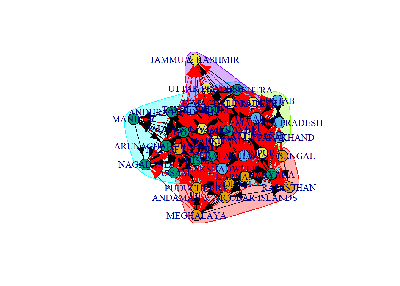

Code

#collect modularity scores to compare
mod_spin_w<-modularity(workto.spin)
mod_spin_w

[1] 0.005774148

Migration due to marriage

The communities identified by the 2 algorithms are quite similar for migrants who move for marriage. The modularity scores (0.16 and 0.09) indicate that the communities are significantly different from what would be expected in a random network.

The walktrap community detection algorithm identified 5 clusters whereas the spinglass algorithm identified 4 clusters. The clusters identified by these two algorithms mostly had states confined to a particular region of India, demonstrating that people do not move farther distances for marriage in comparison to those who moved for work.

The first cluster for both algorithms consist of states from the Southern region of India in addition to the island/union territory- Andaman and Nicobar Islands. Similarly clusters 4 in walktrap and 3 in spinglass have states from the Northern region, with the exception of Puducherry (located in the South) in the cluster identified by Spinglass.

While there were some differences in states, clusters 3 in walktrap and 4 in spinglass represent the North-eastern region whereas clusters 2 for both the algorithms consist of states from Central/Western India.

Walktrap Community Detection

Code

set.seed(20)
#Run clustering algorithm: walktrap
marto.wt<-walktrap.community(mig_mar_ig,weights=NULL)
#Inspect community membership
igraph::groups(marto.wt)

$`1`
[1] "ANDHRA PRADESH"            "KARNATAKA"                
[3] "ANDAMAN & NICOBAR ISLANDS" "TAMIL NADU"               
[5] "KERALA"                   

$`2`
[1] "MAHARASHTRA"    "GUJARAT"        "ODISHA"         "CHHATTISGARH"  
[5] "MADHYA PRADESH" "GOA"            "DAMAN & DIU"   

$`3`
 [1] "WEST BENGAL"          "DADRA & NAGAR HAVELI" "PUDUCHERRY"          
 [4] "TRIPURA"              "RAJASTHAN"            "ASSAM"               
 [7] "UTTAR PRADESH"        "NAGALAND"             "JHARKHAND"           
[10] "BIHAR"                "SIKKIM"               "MIZORAM"             
[13] "MANIPUR"              "MEGHALAYA"           

$`4`
[1] "HIMACHAL PRADESH" "PUNJAB"           "CHANDIGARH"       "NCT OF DELHI"    
[5] "JAMMU & KASHMIR"  "UTTARAKHAND"      "HARYANA"         

$`5`
[1] "ARUNACHAL PRADESH" "LAKSHADWEEP"

Code

#add community membership as a vertex attribute
nodes_m$comm.wt<-marto.wt$membership
#plot the network with community coloring
plot(marto.wt,mig_mar_ig)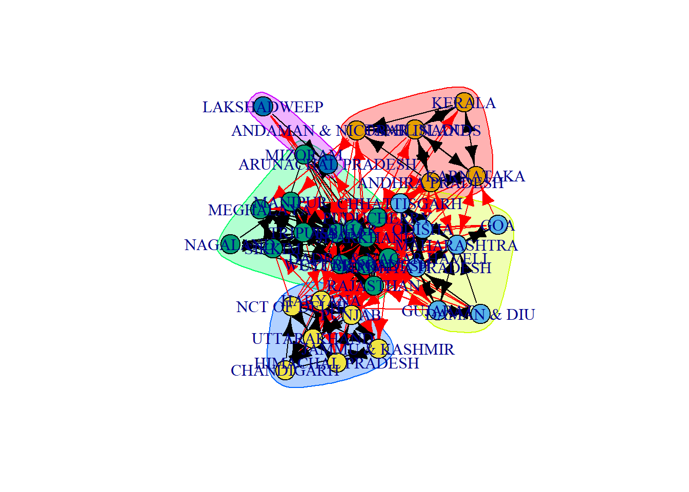

Code

#modularity
mod_m<-modularity(marto.wt)
mod_m

[1] 0.16409

Spinglass

Code

set.seed(20)
#Run clustering algorithm: spinglass
marto.spin<-spinglass.community(mig_mar_ig)
#Inspect community membership
igraph::groups(marto.spin)

$`1`
[1] "ANDHRA PRADESH"            "KARNATAKA"                
[3] "ANDAMAN & NICOBAR ISLANDS" "TAMIL NADU"               
[5] "KERALA"                   

$`2`
 [1] "DADRA & NAGAR HAVELI" "MAHARASHTRA"          "UTTAR PRADESH"       
 [4] "GUJARAT"              "JHARKHAND"            "ODISHA"              
 [7] "CHHATTISGARH"         "MADHYA PRADESH"       "MIZORAM"             
[10] "DAMAN & DIU"         

$`3`
[1] "HIMACHAL PRADESH" "PUNJAB"           "CHANDIGARH"       "NCT OF DELHI"    
[5] "PUDUCHERRY"       "JAMMU & KASHMIR"  "UTTARAKHAND"      "HARYANA"         
[9] "RAJASTHAN"       

$`4`
 [1] "WEST BENGAL"       "TRIPURA"           "ASSAM"            
 [4] "NAGALAND"          "BIHAR"             "SIKKIM"           
 [7] "GOA"               "ARUNACHAL PRADESH" "MANIPUR"          
[10] "MEGHALAYA"         "LAKSHADWEEP"

Code

#add community membership as a vertex attribute
nodes_m$comm.spin<-marto.spin$membership
#plot the network with community coloring
plot(marto.spin,mig_mar_ig)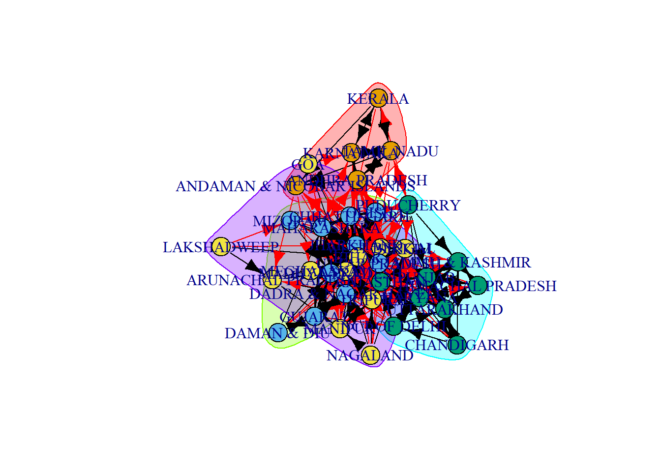

Code

#collect modularity scores to compare
mod_spin_m<-modularity(marto.spin)
mod_spin_m

[1] 0.009442108

Network correlation

I chose to use the QAP test since both my networks had the same nodes but were created with different tie content.

The plot depicts that the differences between the two networks is statistically significant. Moreover, the negative correlation further strengthens the dissimilarity between the migration network for work and migration network for marriage.

Code

gcor(mig_work_stat,mig_mar_stat)

[1] -0.04724667

Code

qap<-qaptest(list(mig_work_stat,mig_mar_stat),gcor,g1=1,g2=2)
qap


QAP Test Results

Estimated p-values:
    p(f(perm) >= f(d)): 0.86 
    p(f(perm) <= f(d)): 0.157

Code

plot(qap, xlim=c(min(qap$dist)-.02, qap$testval+.02))
abline(v=qap$testval, col="red")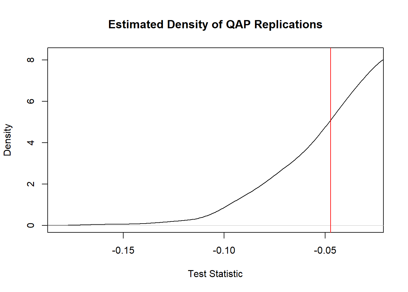

Conclusion

To summarise, there is a difference observed for the patterns of movement for work and marriage. For the threshold considered in the project (at least a proportion of 20%), it is clear that more people move for work than for marriage. Moreover, people moving for work are open to move to multiple geographic regions whereas people moving for marriage mostly move within the same geographic region. The major region of out migration for work was observed to be parts of North and East India but no such major region of in migration for work was found. Finally, several of the top sending states of migrants due to marriage were simultaneously top receiving states of migrants due to marriage.

In future research, this analysis can be extended to the other reasons for migration present in the Census dataset, including but not limited to movement for education, business and within the household. Additionally, it may be interesting to observe if the patterns of movement for a particular reason has changed over years, by incorporating Census data from various time periods. It would also be helpful to study trends in Census data in the 2020-2030 decade when it is released.

References

Bhardwaj, A., & Batra, S. (2022, July 26). No census 2021 in 2022 either - govt ‘puts exercise on hold, timeframe not yet decided’.ThePrint.https://theprint.in/india/no-census-2021-in-2022-either-govt-puts-exercise-on-hold-timeframe-not-yet-decided/1055772/
Government of India. (n.d.).Drop-in-article on census - no.8 (migration).
https://censusindia.gov.in/nada/index.php/catalog/40447
Lumen Learning. (n.d.). Systems of Social Stratification. https://courses.lumenlearning.com/wm-introductiontosociology/chapter/systems-of-social-stratification/
Office of the Registrar General India. (2021). D-03: Migrants within the State/UT by place of last residence, duration of residence and reason of migration - 2011.
[India]. https://censusindia.gov.in/census.website/data/census-tables
Sahgal,N., Evans, J., Salazar, A.M., Starr, K.J. & Corichi, M. (2021, June 29). 4. attitudes about caste. Pew Research Center’s Religion & Public Life Project. https://www.pewresearch.org/religion/2021/06/29/attitudes-about-caste/