WK7Challenge_KDocekal

Code

library(tidyverse)
library(igraph)
library(statnet)
library(gssr)
library(drat)

knitr::opts_chunk$set(echo = TRUE)

My dataset uses results from the 1985 General Social Survey. The 1985 GSS dataset is in edgelist format. There are 1534 observations with 622 variables.

Code

remotes::install_github("kjhealy/gssr")

Skipping install of 'gssr' from a github remote, the SHA1 (abe949b1) has not changed since last install.
  Use `force = TRUE` to force installation

Code

drat::addRepo("kjhealy")

gss85 <- gss_get_yr(1985)

Fetching: https://gss.norc.org/documents/stata/1985_stata.zip

Code

head(
gss85)

# A tibble: 6 × 662
  year     id wrkstat hrs1        hrs2        evwork      occ   prestige wrkslf 
  <dbl> <dbl> <dbl+l> <dbl+lbl>   <dbl+lbl>   <dbl+lbl>   <dbl> <dbl+lb> <dbl+l>
1 1985      1 1 [wor…    40       NA(i) [iap] NA(i) [iap] 194   51       2 [som…
2 1985      2 1 [wor…    65       NA(i) [iap] NA(i) [iap]  31   76       1 [sel…
3 1985      3 2 [wor…     9       NA(i) [iap] NA(i) [iap] 180   51       2 [som…
4 1985      4 3 [wit… NA(i) [iap]    60       NA(i) [iap]  65   82       2 [som…
5 1985      5 1 [wor…    40       NA(i) [iap] NA(i) [iap] 915   20       2 [som…
6 1985      6 1 [wor…    40       NA(i) [iap] NA(i) [iap] 185   46       1 [sel…
# ℹ 653 more variables: wrkgovt <dbl+lbl>, industry <dbl+lbl>, found <dbl+lbl>,
#   occ10 <dbl+lbl>, occindv <dbl+lbl>, occstatus <dbl+lbl>, occtag <dbl+lbl>,
#   prestg10 <dbl+lbl>, prestg105plus <dbl+lbl>, indus10 <dbl+lbl>,
#   indstatus <dbl+lbl>, indtag <dbl+lbl>, marital <dbl+lbl>, agewed <dbl+lbl>,
#   divorce <dbl+lbl>, spwrksta <dbl+lbl>, sphrs1 <dbl+lbl>, sphrs2 <dbl+lbl>,
#   spevwork <dbl+lbl>, spocc <dbl+lbl>, sppres <dbl+lbl>, spwrkslf <dbl+lbl>,
#   spind <dbl+lbl>, spocc10 <dbl+lbl>, spoccindv <dbl+lbl>, …

Code

dim(gss85)

[1] 1534  662

We can first create the dataframe by selecting the ties variable. Here I use “talkto” which provides weighted edges based on members a respondent’s group of contacts. Weights are based on respondents’ perception of how much each contact talks to each other.

Code

ties <- gss85[,grepl("talkto", colnames(gss85))]
head(ties)

# A tibble: 6 × 5
  talkto1             talkto2          talkto3          talkto4      talkto5    
  <dbl+lbl>           <dbl+lbl>        <dbl+lbl>        <dbl+lbl>    <dbl+lbl>  
1 2 [once a week]     1 [almost daily] 3 [once a month] 3 [once a m…     2 [onc…
2 1 [almost daily]    2 [once a week]  1 [almost daily] 1 [almost d…     1 [alm…
3 2 [once a week]     2 [once a week]  2 [once a week]  1 [almost d…     2 [onc…
4 1 [almost daily]    1 [almost daily] 3 [once a month] 2 [once a w…     1 [alm…
5 2 [once a week]     2 [once a week]  3 [once a month] 3 [once a m…     2 [onc…
6 4 [lt once a month] 2 [once a week]  2 [once a week]  1 [almost d… NA(i) [iap]

A matrix and the igraph network can be created using the previous ties. There are 5 rows and columns corresponding to the number of respondent contacts, ties are undirected and weighted.

Code

mat = matrix(nrow = 5, ncol = 5)

mat[lower.tri(mat)] <- as.numeric(ties[3,])

mat[upper.tri(mat)] = t(mat)[upper.tri(mat)]

na_vals <- is.na(mat)
non_missing_rows <- rowSums(na_vals) < nrow(mat)
mat <- mat[non_missing_rows,non_missing_rows]

diag(mat) <- 0

mat

     [,1] [,2] [,3] [,4] [,5]
[1,]    0    2    2    2    1
[2,]    2    0    2    2    2
[3,]    2    2    0    2    1
[4,]    2    2    2    0    2
[5,]    1    2    1    2    0

Code

ig.net <- graph.adjacency(mat, mode = "undirected", weighted = T)

Edges represent the weight between contacts. Contacts are numbered 1-5, based on participants’ response order. For example, Edge 1–2 indicates that contacts number 1 and 2 talk to each other.

Code

print(ig.net)

IGRAPH 20c2069 U-W- 5 10 -- 
+ attr: weight (e/n)
+ edges from 20c2069:
 [1] 1--2 1--3 1--4 1--5 2--3 2--4 2--5 3--4 3--5 4--5

Code

head(ig.net)

5 x 5 sparse Matrix of class "dgCMatrix"
              
[1,] . 2 2 2 1
[2,] 2 . 2 2 2
[3,] 2 2 . 2 1
[4,] 2 2 2 . 2
[5,] 1 2 1 2 .

Results show that there is 1 component and the median weight is 2.

Code

igraph::components(ig.net)$no

[1] 1

Code

summary(E(ig.net)$weight)

   Min. 1st Qu.  Median    Mean 3rd Qu.    Max. 
    1.0     2.0     2.0     1.8     2.0     2.0 

This network contains 5 vertices and 10 edges. Ties are not bipartite or directed but they are weighted.

Code

vcount(ig.net)

[1] 5

Code

ecount(ig.net)

[1] 10

Code

is_bipartite(ig.net)

[1] FALSE

Code

is_directed(ig.net)

[1] FALSE

Code

is_weighted(ig.net)

[1] TRUE

As an undirected graph we can use Fast and Greedy for community clustering.

Code

#Run clustering algorithm: fast_greedy
comm.fg<-cluster_fast_greedy(ig.net)

#Inspect clustering object
names(comm.fg)

[1] "merges"     "modularity" "membership" "algorithm"  "vcount"    

This identifies two groups; contact 3 and all other nodes.

Code

comm.fg

IGRAPH clustering fast greedy, groups: 2, mod: 2.8e-17
+ groups:
  $`1`
  [1] 1 2 4 5
  
  $`2`
  [1] 3
  

Examining the community membership vector shows membership distribution.

Code

comm.fg$membership

[1] 1 1 2 1 1

Plotting with coloring shows a visualization of these two communities.

Code

plot(comm.fg,ig.net)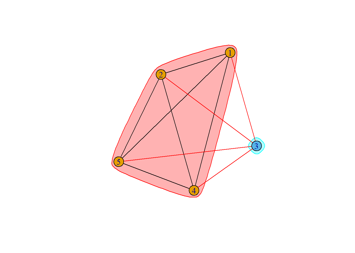

Walktrap is another potential algorithm for community detection.

Code

comm.wt<-walktrap.community(ig.net)


igraph::groups(comm.wt)

$`1`
[1] 1 2 3 4 5

Testing with steps ranging from 20 to 2000 all reveal the same, single community.

Code

igraph::groups(walktrap.community(ig.net ,steps=20))

$`1`
[1] 1 2 3 4 5

Code

igraph::groups(walktrap.community(ig.net ,steps=200))

$`1`
[1] 1 2 3 4 5

Code

igraph::groups(walktrap.community(ig.net ,steps=2000))

$`1`
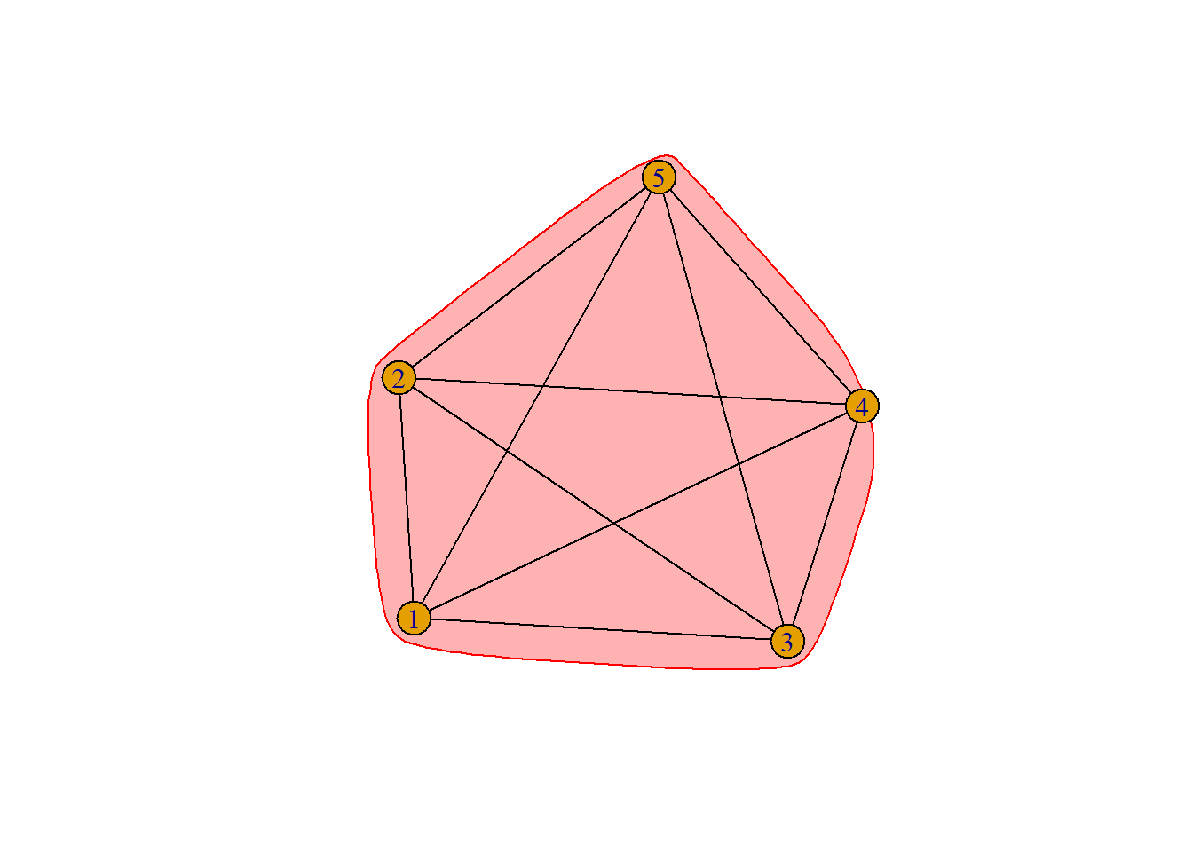
[1] 1 2 3 4 5

Plotting the network with Walktrap shows a single community with all nodes connected. The walktrap community makes the most sense as the more representative graph as we already know nodes are connected through their association with the respondent. In this case changing the number of steps does affect theses results and confirms our expectations.

Code

plot(comm.wt,ig.net)