Blog Post #2: Gathering Data

Setup

View Code

Code

library(tidyverse)

── Attaching packages ─────────────────────────────────────── tidyverse 1.3.1 ──

✔ ggplot2 3.3.6     ✔ purrr   0.3.4
✔ tibble  3.1.7     ✔ dplyr   1.0.9
✔ tidyr   1.2.0     ✔ stringr 1.4.1
✔ readr   2.1.2     ✔ forcats 0.5.1

── Conflicts ────────────────────────────────────────── tidyverse_conflicts() ──
✖ dplyr::filter() masks stats::filter()
✖ dplyr::lag()    masks stats::lag()

Code

library(tidytext)
library(readr)
library(devtools)

Loading required package: usethis

Code

library(plyr)

------------------------------------------------------------------------------

You have loaded plyr after dplyr - this is likely to cause problems.
If you need functions from both plyr and dplyr, please load plyr first, then dplyr:
library(plyr); library(dplyr)

------------------------------------------------------------------------------

Attaching package: 'plyr'

The following objects are masked from 'package:dplyr':

    arrange, count, desc, failwith, id, mutate, rename, summarise,
    summarize

The following object is masked from 'package:purrr':

    compact

Code

library(knitr)
library(rvest)

Attaching package: 'rvest'

The following object is masked from 'package:readr':

    guess_encoding

Code

library(rtweet)

Attaching package: 'rtweet'

The following object is masked from 'package:purrr':

    flatten

Code

library(twitteR)

Attaching package: 'twitteR'

The following object is masked from 'package:rtweet':

    lookup_statuses

The following object is masked from 'package:plyr':

    id

The following objects are masked from 'package:dplyr':

    id, location

Code

library(tm)

Loading required package: NLP

Attaching package: 'NLP'

The following object is masked from 'package:ggplot2':

    annotate

Code

library(lubridate)

Attaching package: 'lubridate'

The following objects are masked from 'package:base':

    date, intersect, setdiff, union

Code

library(quanteda)

Warning in .recacheSubclasses(def@className, def, env): undefined subclass
"unpackedMatrix" of class "mMatrix"; definition not updated

Warning in .recacheSubclasses(def@className, def, env): undefined subclass
"unpackedMatrix" of class "replValueSp"; definition not updated

Package version: 3.2.3
Unicode version: 13.0
ICU version: 69.1

Parallel computing: 6 of 6 threads used.

See https://quanteda.io for tutorials and examples.

Attaching package: 'quanteda'

The following object is masked from 'package:tm':

    stopwords

The following objects are masked from 'package:NLP':

    meta, meta<-

Code

library(quanteda.textplots)
knitr::opts_chunk$set(echo = TRUE)

Data Sources

For this assignment, I gathered the data for my corpus from the Twitter social media platform. The ‘rtweet’ R package was used heavily in the gathering and preliminary analysis of the data I used. In order to extract twitter data to R, I needed to first create a developer account to gain the appropriate permissions. Once the account was made, I was able to create a new project through the developer app and connect it to R. From there, I was able to begin gathering data and conducting a preliminary analysis of what I could find so far.

Gathering Data

The first step in data analysis, is gathering the data you intend to analyze! I started by gathering as many tweets as possible related to the subject of my project. At this point, the goal of my project is to conduct a sentiment analysis surrounding the perception of eating insects among twitter users. So, I pulled tweets containing the keywords eating and bugs/insects. Finding it unnecessary, I excluded re-tweets and chose to restrict source language to only those in English.

Code

#Pull together tweets containing keywords 'eating` and `bugs/insects`.
tweet_bugs <- search_tweets("eating bugs OR insects", n = 10000,
                             type = "mixed",
                             include_rts = FALSE,
                             lang = "en")

Creating a Corpus

From the previous chunk, I was able to gather a total of 1,533 tweets along with their metadata. The following chunk is dedicated toward cleaning up the data a bit and pulling out the information I need in order to conduct the analysis. First I extracted the full_text column from the tweet_bugs object I created and stored it as tweet_text. From there, I converted the text object to a corpus, i.e. tweet_corpus. Lastly, I used the summary function to summarize corpus information like sentence and token count per tweet (for some reason, the summary function limited itself to only 100 out of the 1,533 entries. A goal for the future is to figure out how to extend it so that I can summarize the full corpus data).

Code

#Separate out the text from tweet_bugs and build the corpus.
tweet_text <- as.vector.data.frame(tweet_bugs$full_text, mode = "any")
tweet_corpus <- corpus(tweet_text)
tweet_summary <- summary(tweet_corpus)

While not entirely useful, I also decided to add in a tweet count indicator to number the tweets. Once again, the count only extended up to the first 100 entries. Hopefully, there is a workaround to include the remainder of the entries, but ultimately it isn’t crucial when conducting sentiment analysis.

View Code

Code

#Creating tweet count indicator (i.e. Count).
tweet_summary$Count <- as.numeric(str_extract(tweet_summary$Text,"[0-9]+"))
tweet_summary

Corpus consisting of 957 documents, showing 100 documents:

    Text Types Tokens Sentences Count
   text1    14     14         1     1
   text2    43     51         3     2
   text3    41     52         1     3
   text4    47     55         2     4
   text5    48     56         4     5
   text6    29     32         1     6
   text7    17     24         2     7
   text8    48     60         4     8
   text9    14     16         2     9
  text10    44     53         7    10
  text11    28     29         3    11
  text12    20     22         1    12
  text13    54     65         3    13
  text14    13     13         1    14
  text15    29     32         1    15
  text16    42     45         1    16
  text17    49     59         3    17
  text18    13     13         1    18
  text19    32     38         1    19
  text20    13     14         1    20
  text21    45     65         7    21
  text22    24     27         2    22
  text23    31     41         4    23
  text24    42     48         3    24
  text25    15     15         1    25
  text26    31     36         4    26
  text27    45     57         3    27
  text28    57     61         4    28
  text29     8      9         1    29
  text30    38     48         3    30
  text31    15     15         1    31
  text32    14     14         1    32
  text33    22     24         3    33
  text34     9      9         1    34
  text35     5      5         1    35
  text36    47     52         6    36
  text37    15     15         1    37
  text38    26     30         3    38
  text39    21     21         1    39
  text40    21     22         1    40
  text41     9     13         1    41
  text42    23     29         3    42
  text43    28     37         1    43
  text44    15     16         1    44
  text45    40     48         1    45
  text46    28     35         3    46
  text47    18     26         4    47
  text48    28     29         1    48
  text49    17     18         1    49
  text50    43     58         1    50
  text51    25     28         1    51
  text52    39     49         1    52
  text53    14     17         4    53
  text54    39     51         3    54
  text55    48     58         2    55
  text56    22     28         1    56
  text57    46     53         4    57
  text58    17     21         1    58
  text59    12     12         1    59
  text60    41     45         3    60
  text61    11     11         1    61
  text62    25     26         2    62
  text63    32     34         4    63
  text64    13     14         1    64
  text65     9     12         3    65
  text66     7      7         1    66
  text67    27     32         1    67
  text68    38     42         3    68
  text69    34     36         2    69
  text70    10     10         1    70
  text71    28     30         1    71
  text72    13     13         1    72
  text73    56     61         4    73
  text74    34     41         4    74
  text75    43     59         5    75
  text76    22     24         2    76
  text77    29     33         2    77
  text78    32     34         1    78
  text79     9      9         1    79
  text80    33     39         1    80
  text81    41     46         3    81
  text82    11     12         2    82
  text83    20     21         1    83
  text84    42     46         3    84
  text85    30     34         2    85
  text86    21     31         3    86
  text87    22     28         2    87
  text88    10     10         1    88
  text89    21     24         4    89
  text90    37     52         3    90
  text91     7      7         1    91
  text92    26     29         1    92
  text93     9      9         1    93
  text94    41     50         4    94
  text95    12     13         1    95
  text96    44     48         2    96
  text97    41     45         3    97
  text98    10     10         1    98
  text99     8      8         1    99
 text100    37     43         3   100

Additionally, because Twitter’s base developer guidelines only allow me to extract tweets created within the last 6-9 days, I tried to pull as many within this time frame as possible and write them to a csv document for storage. My hope is that as my project progresses, I can accumulate and append additional tweets to my existing corpus so that by the end I have a larger data frame to work with.

Code

#Creating a new document to store existing corpus and hopefully add more over time.
write.csv(tweet_corpus, file = "eating_bugs_tweets_11_3_22.csv", row.names = FALSE)

Preliminary Analysis

Beginning my analysis of the data, I decided to run the docvars function to check for metadata (which after extracting the text column from the the initial tweet_bugs object, I figured would no longer include any).

View Code

Code

#Trying to pull metadata, but there no longer is any.
docvars(tweet_corpus)

data frame with 0 columns and 957 rows

Afterwards, I decided to split the corpus down into sentence level documents. I thought that by doing this, I would be able to call back to this object eventually and analyze sentiment within each individual sentence, but I realized and felt as though this spread my data a bit too thin and thought that it would be better to split it down to the tweet level (documents) instead. That way, I can consolidate the data a bit and effectively analyze the sentiment of the person behind each individual tweet.

View Code

Code

#These lines of code separate out each sentence within the tweet corpus. Only problem was, many tweets contained multiple sentences and this spreads the data very thin.
ndoc(tweet_corpus)

[1] 957

Code

tweet_corpus_sentences <- corpus_reshape(tweet_corpus, to = "sentences")
ndoc(tweet_corpus_sentences)

[1] 2051

Code

#From there, I instead decided to separate them by tweet, i.e. document, to get a better idea of each individuals writing style and opinion. I felt as though 'sentences' was spreading it too thin.
tweet_corpus_document <- corpus_reshape(tweet_corpus, to = "documents")
ndoc(tweet_corpus_document)

[1] 957

Code

summary(tweet_corpus_document, n=5)

Corpus consisting of 957 documents, showing 5 documents:

  Text Types Tokens Sentences
 text1    14     14         1
 text2    43     51         3
 text3    41     52         1
 text4    47     55         2
 text5    48     56         4

Tokens

Next I decided break the corpus down to the token level and conduct a surface level analysis on the use of certain keywords. The following code chunk is indicative of my thought process when creating the tweet_token object. First, I created the base object, then removed any punctuation, and finally removed all numbers.

View Code

Code

#My next step was to tokenize the corpus. The initial 'token' code uses the base tokenizer which breaks on white space.  
tweet_tokens <- tokens(tweet_corpus)
print(tweet_tokens)

Tokens consisting of 957 documents.
text1 :
 [1] "Surging"      "populations"  "of"           "plant-eating" "insects"     
 [6] "are"          "disrupting"   "farms"        "and"          "the"         
[11] "food"         "supply"      
[ ... and 2 more ]

text2 :
 [1] "If"       "he"       "had"      "any"      "respect"  "for"     
 [7] "bereaved" "families" ","        "he"       "would"    "be"      
[ ... and 39 more ]

text3 :
 [1] "Covid-19"     "Bereaved"     "Families"     "for"          "Justice"     
 [6] "says"         "Matt"         "Hancock"      "should"       "be"          
[11] "co-operating" "with"        
[ ... and 40 more ]

text4 :
 [1] "Entertainment" "show"          "with"          "so"           
 [5] "called"        "celebrities"   "A"             "gov"          
 [9] "minister"      "whos"          "gov"           "is"           
[ ... and 43 more ]

text5 :
 [1] "@Joshua_Griffing" "@Bulletsnbrains"  "@runninvsthewind" "@iluminatibot"   
 [5] "Dude"             "."                "."                "."               
 [9] "Those"            "are"              "tweets"           "from"            
[ ... and 44 more ]

text6 :
 [1] "Most"     "people"   "think"    "that"     "eating"   "insects" 
 [7] "and"      "eating"   "crabs"    "/"        "lobsters" "is"      
[ ... and 20 more ]

[ reached max_ndoc ... 951 more documents ]

Code

#This line of code drops punctuation along with the default space breaks.
tweet_tokens <- tokens(tweet_corpus,
                        remove_punct = T)
print(tweet_tokens)

Tokens consisting of 957 documents.
text1 :
 [1] "Surging"      "populations"  "of"           "plant-eating" "insects"     
 [6] "are"          "disrupting"   "farms"        "and"          "the"         
[11] "food"         "supply"      
[ ... and 2 more ]

text2 :
 [1] "If"       "he"       "had"      "any"      "respect"  "for"     
 [7] "bereaved" "families" "he"       "would"    "be"       "sharing" 
[ ... and 33 more ]

text3 :
 [1] "Covid-19"     "Bereaved"     "Families"     "for"          "Justice"     
 [6] "says"         "Matt"         "Hancock"      "should"       "be"          
[11] "co-operating" "with"        
[ ... and 33 more ]

text4 :
 [1] "Entertainment" "show"          "with"          "so"           
 [5] "called"        "celebrities"   "A"             "gov"          
 [9] "minister"      "whos"          "gov"           "is"           
[ ... and 40 more ]

text5 :
 [1] "@Joshua_Griffing" "@Bulletsnbrains"  "@runninvsthewind" "@iluminatibot"   
 [5] "Dude"             "Those"            "are"              "tweets"          
 [9] "from"             "officials"        "there"            "There"           
[ ... and 35 more ]

text6 :
 [1] "Most"     "people"   "think"    "that"     "eating"   "insects" 
 [7] "and"      "eating"   "crabs"    "lobsters" "is"       "a"       
[ ... and 16 more ]

[ reached max_ndoc ... 951 more documents ]

Code

#This last line of code drops numbers within the token corpus as well.
tweet_tokens <- tokens(tweet_corpus,
                        remove_punct = T,
                        remove_numbers = T)
print(tweet_tokens)

Tokens consisting of 957 documents.
text1 :
 [1] "Surging"      "populations"  "of"           "plant-eating" "insects"     
 [6] "are"          "disrupting"   "farms"        "and"          "the"         
[11] "food"         "supply"      
[ ... and 2 more ]

text2 :
 [1] "If"       "he"       "had"      "any"      "respect"  "for"     
 [7] "bereaved" "families" "he"       "would"    "be"       "sharing" 
[ ... and 31 more ]

text3 :
 [1] "Covid-19"     "Bereaved"     "Families"     "for"          "Justice"     
 [6] "says"         "Matt"         "Hancock"      "should"       "be"          
[11] "co-operating" "with"        
[ ... and 33 more ]

text4 :
 [1] "Entertainment" "show"          "with"          "so"           
 [5] "called"        "celebrities"   "A"             "gov"          
 [9] "minister"      "whos"          "gov"           "is"           
[ ... and 40 more ]

text5 :
 [1] "@Joshua_Griffing" "@Bulletsnbrains"  "@runninvsthewind" "@iluminatibot"   
 [5] "Dude"             "Those"            "are"              "tweets"          
 [9] "from"             "officials"        "there"            "There"           
[ ... and 35 more ]

text6 :
 [1] "Most"     "people"   "think"    "that"     "eating"   "insects" 
 [7] "and"      "eating"   "crabs"    "lobsters" "is"       "a"       
[ ... and 14 more ]

[ reached max_ndoc ... 951 more documents ]

After creating the tweet_tokens object, I searched through the corpus for the keywords using the kwic function. The first use of the function in the chunk below searched for the use of the keywords bug & bugs, while the second analyzes the words insect & insects. I decided to open up the window to 20 words surrounding the keywords (i.e. patterns). I felt this gave me a sufficient window to, at a glance, gauge sentiment within the use of the words.

Code

#These lines of code are dedicated toward the analysis of tokens on a more granular level. This first blurb is analyzing the use of the keywords 'bug' & 'bugs' within the corpus.
kwic_bugs <- kwic(tweet_tokens,
                   pattern = c("bug", "bugs"),
                   window = 20)
view(kwic_bugs)

#This second blurb analyzes the use of the keywords 'insect' & 'insects' instead.
kwic_insects <- kwic(tweet_tokens, 
                   pattern = c("insect", "insects"),
                   window = 20)
view(kwic_insects)

I noticed throughout the corpus that the specified keywords were often surrounded by argument and context provided by the individual tweeting them. This is what eventually led me to open the window to 20 words. I also noticed that there were a lot of advertisement campaigns based upon the concept of promoting ones channel/profile by eating bugs. Similarly, there were also some occurrences where the topic of eating bugs was brought up as it relates to nature (for example, bats eating insects and other animal diets) and not according to human dietary habits. I hope that I will be able to further clean up the corpus in future iterations of my project and blog post, consolidating the information further will definitely help me get better results.

With that said, there were plenty of entries relating to the perspective surrounding humans eating bugs. Many were in relation to political ideologies as well and from a bird’s eye view, I noticed a relatively even dispersion of positive and negative opinions surrounding the topic (although, I feel like the average leaned a bit more toward the negative). My goal in the future would be to use dictionary functions to conduct a legitimate sentiment analysis and see how the use of the keywords appear in proportionality of positive vs. negative uses.

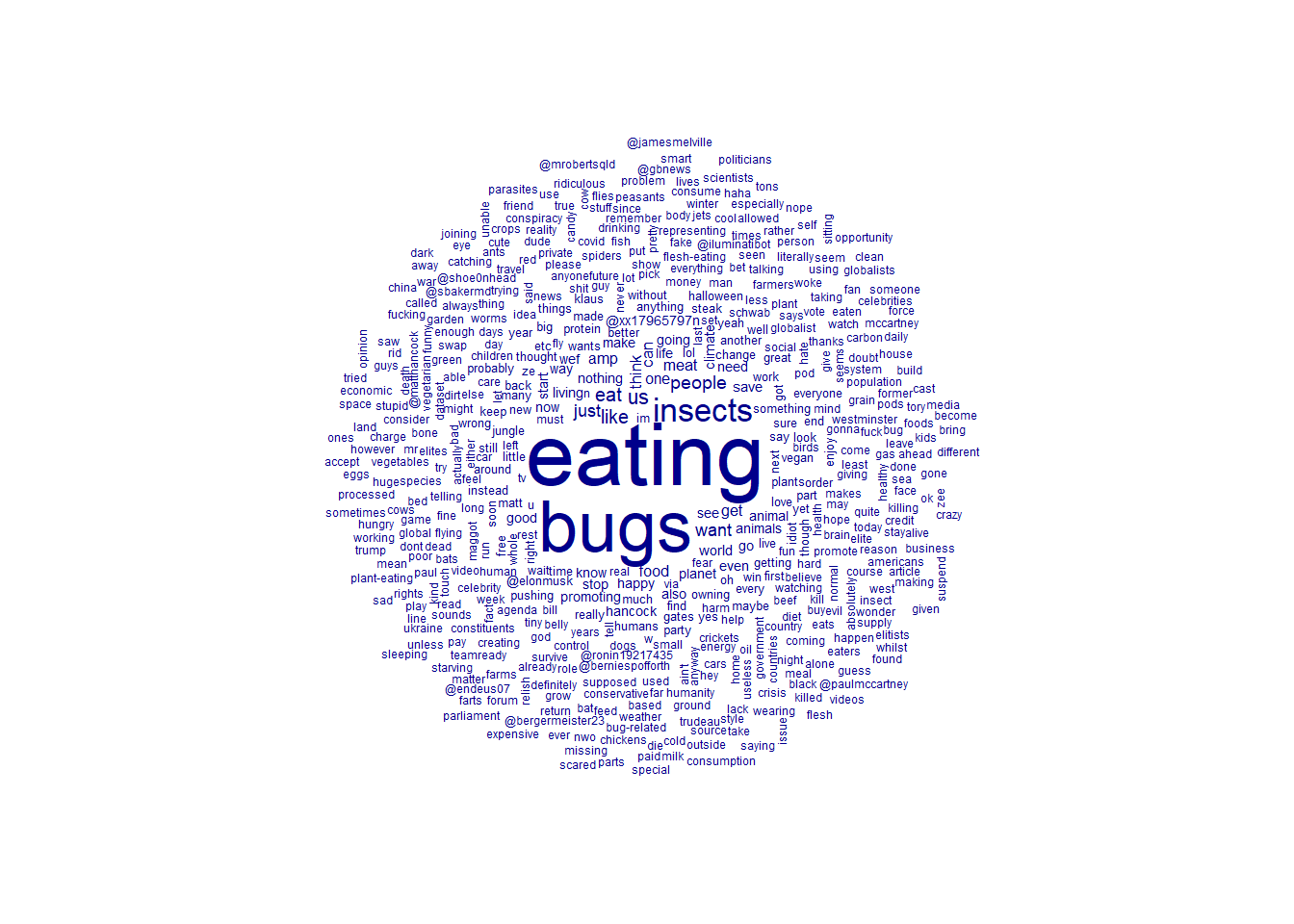
Word Cloud

That last thing I attempted was creating a word cloud using the basis of tokenization that I presented in the previous subsection. Please note, effectively, I could have just used the tweet_token object here instead tweet_corpus, but I wanted to show the thought process of creating a word cloud and practice the syntax behind the relevant functions.

Code

#Creating a dfm that we'll use to create a wordcloud to try and obtain a birds eye view of word usage throughout our corpus.
tweet_dfm <- tokens(tweet_corpus, 
                     remove_punct = TRUE,
                     remove_numbers = TRUE,
                     remove_symbols = TRUE,
                     remove_url = TRUE) %>%
                             tokens_select(pattern = stopwords("en"),
                                           selection = "remove") %>%
                             dfm()
textplot_wordcloud(tweet_dfm)

Unfortunately, I couldn’t take away much from creating the wordcloud. Observably, ‘eating’, ‘insects’ and ‘bugs’ were the most common words, but nothing else in the cloud stood out much or held any real significance. I also noticed that twitter handles and other ‘@s’ still appeared even though I thought I cut them out with the ‘remove_symbols’ function. A goal in the future will be to cut down further language that might be considered disruptive to the analysis.