Blog Post 4: Sentiment analysis

Code

#loading in nececssary libraries
library(quanteda.sentiment)

Loading required package: quanteda

Package version: 3.2.3
Unicode version: 13.0
ICU version: 69.1

Parallel computing: 8 of 8 threads used.

See https://quanteda.io for tutorials and examples.

Attaching package: 'quanteda.sentiment'

The following object is masked from 'package:quanteda':

    data_dictionary_LSD2015

Code

library(quanteda)
library(tidyr)
library(dplyr)

Attaching package: 'dplyr'

The following objects are masked from 'package:stats':

    filter, lag

The following objects are masked from 'package:base':

    intersect, setdiff, setequal, union

Code

library(ggplot2)
library(devtools)

Loading required package: usethis

Code

library(RCurl)

Attaching package: 'RCurl'

The following object is masked from 'package:tidyr':

    complete

Code

#devtools::install_github("kbenoit/quanteda.dictionaries")
library(quanteda.dictionaries)
#remotes::install_github("quanteda/quanteda.sentiment")
library(quanteda.sentiment)

For this blog, I wanted to report on my progress trying out sentiment analysis on my data. In my project, my corpus is made up of speeches given by world leaders at the UN climate change conferences (COP1 - COP15). First, I prepared the data, and ran sentiment analysis.

Code

#loading in the processed dataset. 
x <- getURL('https://raw.githubusercontent.com/andrea-yj-mah/DatafilesTAD/main/FINAL_combined_meta-text_dataset.csv')
speechdf <- read.csv(text = x)

#convert the data to a corpus
speech_corpus <- corpus(speechdf)

#run sentiment analysis
speech_nrc_sentiment <- liwcalike(speech_corpus, data_dictionary_NRC)

Warning in nsentence.character(as.character(x)): nsentence() does not correctly
count sentences in all lower-cased text

Code

#check output
head(speech_nrc_sentiment)

  docname Segment  WPS   WC Sixltr   Dic anger anticipation disgust fear  joy
1   text1       1  597  597  23.45 24.79  0.17         2.18    0.17 2.35 2.68
2   text2       2 2626 2626  34.23 20.11  0.34         2.36    0.30 1.49 1.18
3   text3       3 1141 1141  35.67 22.17  0.44         2.63    0.35 3.07 1.84
4   text4       4  621  621  37.84 19.65  0.81         1.77    0.16 1.61 0.97
5   text5       5  726  726  37.74 26.86  0.83         1.93    0.83 2.20 1.52
6   text6       6 1300 1300  38.00 22.38  0.08         2.00    0.15 2.23 1.31
  negative positive sadness surprise trust AllPunc Period Comma Colon SemiC
1     0.67     8.88    0.50     0.84  6.37    0.00      0     0     0     0
2     1.07     7.04    0.53     0.69  5.10    0.27      0     0     0     0
3     1.49     7.89    0.35     0.79  3.33    0.53      0     0     0     0
4     1.13     9.34    0.48     0.16  3.22    0.32      0     0     0     0
5     1.93    11.16    1.10     0.41  4.96    0.96      0     0     0     0
6     1.08     9.38    0.69     0.31  5.15    0.08      0     0     0     0
  QMark Exclam Dash Quote Apostro Parenth OtherP
1     0      0    0  0.00       0       0   0.00
2     0      0    0  0.27       0       0   0.27
3     0      0    0  0.53       0       0   0.53
4     0      0    0  0.32       0       0   0.32
5     0      0    0  0.96       0       0   0.96
6     0      0    0  0.08       0       0   0.08

Code

# converting the corpus to dfm using the dictionary
speech_nrc <- tokens(speech_corpus,
                             include_docvars = TRUE) %>%
  dfm() %>%
  dfm_lookup(data_dictionary_NRC)

#checking the conversion and outputs
dim(speech_nrc)

[1] 1260   10

Code

head(speech_nrc, 10)

Document-feature matrix of: 10 documents, 10 features (0.00% sparse) and 10 docvars.
       features
docs    anger anticipation disgust fear joy negative positive sadness surprise
  text1     1           13       1   14  16        4       53       3        5
  text2     9           62       8   39  31       28      185      14       18
  text3     5           30       4   35  21       17       90       4        9
  text4     5           11       1   10   6        7       58       3        1
  text5     6           14       6   16  11       14       81       8        3
  text6     1           26       2   29  17       14      122       9        4
       features
docs    trust
  text1    38
  text2   134
  text3    38
  text4    20
  text5    36
  text6    67
[ reached max_ndoc ... 4 more documents ]

Code

class(speech_nrc)

[1] "dfm"
attr(,"package")
[1] "quanteda"

After running the inital sentiment analysis, I had a dfm, but the dfm was missing my metadata, and I couldn’t use the dfm to run calculations that I was interested in. I calculated polarity by document. Next, I converted the dfm to a data frame object and merged it with my metadata.

Code

#converting the data to a dataframe to be able to perform calculations. 
df_nrc <- convert(speech_nrc, to = "data.frame")

#calculate polarity like we learned in class
df_nrc$polarity <- (df_nrc$positive - df_nrc$negative)/(df_nrc$positive + df_nrc$negative)

df_nrc$polarity[(df_nrc$positive + df_nrc$negative) == 0] <- 0

#now I want to merge it back with the dataframe that has all the metadata
names(speechdf)

 [1] "X"           "textnum"     "filename"    "year"        "speaker"    
 [6] "File"        "text"        "text_field"  "docid_field" "country"    
[11] "CRI"        

Code

names(df_nrc)

 [1] "doc_id"       "anger"        "anticipation" "disgust"      "fear"        
 [6] "joy"          "negative"     "positive"     "sadness"      "surprise"    
[11] "trust"        "polarity"    

Code

#creating a variable that can help to match data
speechdf$doc_id <- paste("text",speechdf$textnum, sep = "")

#joining the data
df_nrc_meta <- left_join(speechdf, df_nrc, by = "doc_id")

Then I just wanted to look at some descriptive information about the results of the sentiment analysis…I noticed that the mean ‘positive’ scores were a lot higher than those for ‘negative.’ I was curious if the difference was significant and ran some t.tests to see. The speeches contained significantly more positive sentiment than negative. Perhaps this isn’t surprising given that the context where speeches are delivered is one of global cooperation, and probably leaders don’t want to project too much negativity?

Code

summary(df_nrc_meta)

       X             textnum         filename              year     
 Min.   :   1.0   Min.   :   1.0   Length:1260        Min.   :1995  
 1st Qu.: 315.8   1st Qu.: 315.8   Class :character   1st Qu.:1998  
 Median : 630.5   Median : 630.5   Mode  :character   Median :2003  
 Mean   : 630.5   Mean   : 630.5                      Mean   :2003  
 3rd Qu.: 945.2   3rd Qu.: 945.2                      3rd Qu.:2007  
 Max.   :1260.0   Max.   :1260.0                      Max.   :2009  
                                                                    
   speaker              File               text            text_field       
 Length:1260        Length:1260        Length:1260        Length:1260       
 Class :character   Class :character   Class :character   Class :character  
 Mode  :character   Mode  :character   Mode  :character   Mode  :character  
                                                                            
                                                                            
                                                                            
                                                                            
 docid_field          country               CRI            doc_id         
 Length:1260        Length:1260        Min.   :  7.17   Length:1260       
 Class :character   Class :character   1st Qu.: 52.00   Class :character  
 Mode  :character   Mode  :character   Median : 75.17   Mode  :character  
                                       Mean   : 82.58                     
                                       3rd Qu.:111.83                     
                                       Max.   :173.67                     
                                       NA's   :353                        
     anger         anticipation       disgust            fear       
 Min.   : 0.000   Min.   :  0.00   Min.   : 0.000   Min.   :  0.00  
 1st Qu.: 3.000   1st Qu.: 11.00   1st Qu.: 1.000   1st Qu.: 11.00  
 Median : 5.000   Median : 16.00   Median : 3.000   Median : 16.00  
 Mean   : 6.283   Mean   : 18.41   Mean   : 3.757   Mean   : 19.28  
 3rd Qu.: 8.000   3rd Qu.: 23.00   3rd Qu.: 5.000   3rd Qu.: 24.00  
 Max.   :77.000   Max.   :145.00   Max.   :68.000   Max.   :198.00  
                                                                    
      joy            negative         positive         sadness       
 Min.   :  0.00   Min.   :  0.00   Min.   :  1.00   Min.   :  0.000  
 1st Qu.:  7.00   1st Qu.:  8.00   1st Qu.: 42.00   1st Qu.:  3.000  
 Median : 11.00   Median : 14.00   Median : 59.00   Median :  5.000  
 Mean   : 12.89   Mean   : 17.08   Mean   : 67.44   Mean   :  6.834  
 3rd Qu.: 16.00   3rd Qu.: 21.00   3rd Qu.: 81.00   3rd Qu.:  9.000  
 Max.   :148.00   Max.   :247.00   Max.   :491.00   Max.   :128.000  
                                                                     
    surprise          trust           polarity      
 Min.   : 0.000   Min.   :  0.00   Min.   :-0.7500  
 1st Qu.: 2.000   1st Qu.: 26.00   1st Qu.: 0.5067  
 Median : 4.000   Median : 37.00   Median : 0.6195  
 Mean   : 5.207   Mean   : 41.53   Mean   : 0.6044  
 3rd Qu.: 7.000   3rd Qu.: 50.00   3rd Qu.: 0.7193  
 Max.   :50.000   Max.   :368.00   Max.   : 1.0000  
                                                    

Code

t.test(df_nrc_meta$positive, df_nrc_meta$negative, paired = TRUE)

    Paired t-test

data:  df_nrc_meta$positive and df_nrc_meta$negative
t = 54.985, df = 1259, p-value < 2.2e-16
alternative hypothesis: true mean difference is not equal to 0
95 percent confidence interval:
 48.56271 52.15633
sample estimates:
mean difference 
       50.35952 

Moving on to some other analyses with my metadata…

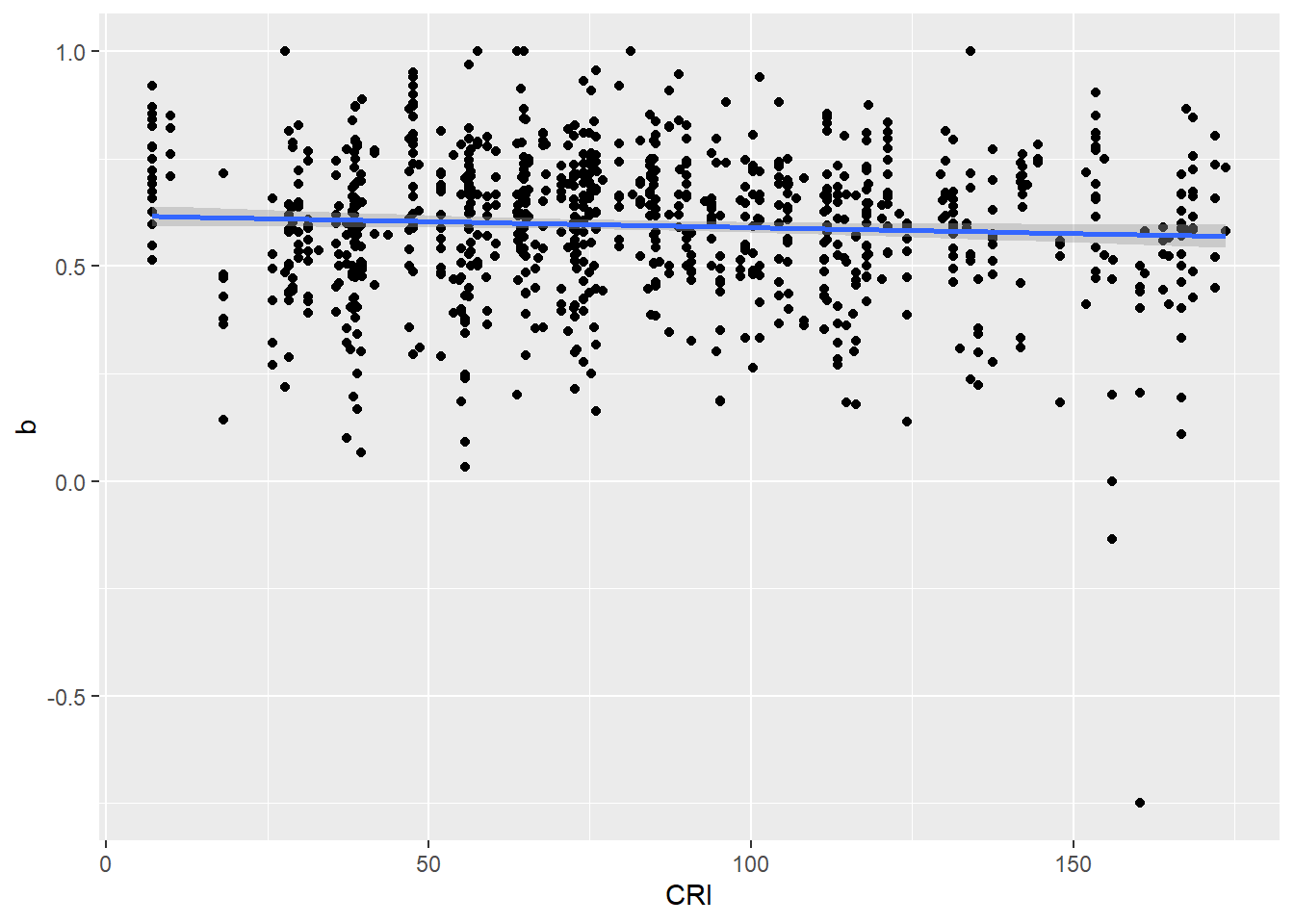
For now, I was interested in two meta-data variables and their relationship to sentiment in the text. These are the year the speech was delivered and the climate risk index (CRI) associated with the country of the speaker. The CRI is based on experienced weather-related impacts on regions/countries like heat-waves, flooding, or storms. Countries with higher CRI are objectively more impacted by climate change. My prediction was that countries with higher CRI may feel more urgency about addressing climate change, and perhaps speeches delivered by members of these countries would contain more negative sentiments, fear, or anger…

Regarding the year speeches were delivered, my thought was that while speeches from the beginning of these conferences would contain more positive sentiments, but that perhaps these decreased over time as climate change impacts became more frequent/severe, and as progress continued to be slow.

For each of these variables, I looked first at correlations and then regressions for any of the observed sigificant correlations. I looked at their relationship to polarity, and then to each of the emotions.

Code

#first, is polarity of speeches associated with year? 
cor.test(df_nrc_meta$year, df_nrc_meta$polarity, method = "pearson")

    Pearson's product-moment correlation

data:  df_nrc_meta$year and df_nrc_meta$polarity
t = -2.1297, df = 1258, p-value = 0.03339
alternative hypothesis: true correlation is not equal to 0
95 percent confidence interval:
 -0.114782383 -0.004727295
sample estimates:
        cor 
-0.05993698 

Code

#second, was polarity of speeches associated with CRI? 
cor.test(df_nrc_meta$CRI, df_nrc_meta$polarity, method = "pearson")

    Pearson's product-moment correlation

data:  df_nrc_meta$CRI and df_nrc_meta$polarity
t = -1.9996, df = 905, p-value = 0.04584
alternative hypothesis: true correlation is not equal to 0
95 percent confidence interval:
 -0.13085287 -0.00123261
sample estimates:
        cor 
-0.06632254 

Both CRI and year were significantly and negatively correlated with polarity.

For yearpolarity: From the beginning of COP conferences –> COP 15, later speeches tended to be more negative For CRIpolarity: Countries who experienced more impacts from climate change tended to give more negative speeches.

Next, I was interested in looking at other emotions. First, I looked at correlations.

Code

cor.emo.year <- function(b){
  cor.test(df_nrc_meta$year, b, method = "pearson")
}
cor.emo.year(df_nrc_meta$fear)

    Pearson's product-moment correlation

data:  df_nrc_meta$year and b
t = 2.6565, df = 1258, p-value = 0.007995
alternative hypothesis: true correlation is not equal to 0
95 percent confidence interval:
 0.01954463 0.12938102
sample estimates:
       cor 
0.07468935 

Code

cor.emo.year(df_nrc_meta$negative)

    Pearson's product-moment correlation

data:  df_nrc_meta$year and b
t = 0.16257, df = 1258, p-value = 0.8709
alternative hypothesis: true correlation is not equal to 0
95 percent confidence interval:
 -0.05065474  0.05979362
sample estimates:
        cor 
0.004583416 

Code

cor.emo.year(df_nrc_meta$positive)

    Pearson's product-moment correlation

data:  df_nrc_meta$year and b
t = -1.843, df = 1258, p-value = 0.06557
alternative hypothesis: true correlation is not equal to 0
95 percent confidence interval:
 -0.106810215  0.003343952
sample estimates:
        cor 
-0.05189097 

Code

cor.emo.year(df_nrc_meta$anger)

    Pearson's product-moment correlation

data:  df_nrc_meta$year and b
t = 2.0953, df = 1258, p-value = 0.03634
alternative hypothesis: true correlation is not equal to 0
95 percent confidence interval:
 0.003760639 0.113828340
sample estimates:
       cor 
0.05897373 

Code

cor.emo.year(df_nrc_meta$disgust)

    Pearson's product-moment correlation

data:  df_nrc_meta$year and b
t = 0.41644, df = 1258, p-value = 0.6772
alternative hypothesis: true correlation is not equal to 0
95 percent confidence interval:
 -0.04351311  0.06692238
sample estimates:
       cor 
0.01174043 

Code

cor.emo.year(df_nrc_meta$surprise)

    Pearson's product-moment correlation

data:  df_nrc_meta$year and b
t = 1.0788, df = 1258, p-value = 0.2809
alternative hypothesis: true correlation is not equal to 0
95 percent confidence interval:
 -0.02486488  0.08548402
sample estimates:
       cor 
0.03040221 

Code

cor.emo.year(df_nrc_meta$trust)

    Pearson's product-moment correlation

data:  df_nrc_meta$year and b
t = -2.082, df = 1258, p-value = 0.03754
alternative hypothesis: true correlation is not equal to 0
95 percent confidence interval:
 -0.113458116 -0.003385576
sample estimates:
        cor 
-0.05859995 

Code

cor.emo.year(df_nrc_meta$anticipation)

    Pearson's product-moment correlation

data:  df_nrc_meta$year and b
t = -0.10984, df = 1258, p-value = 0.9126
alternative hypothesis: true correlation is not equal to 0
95 percent confidence interval:
 -0.05831224  0.05213738
sample estimates:
         cor 
-0.003096873 

Code

cor.emo.year(df_nrc_meta$sadness)

    Pearson's product-moment correlation

data:  df_nrc_meta$year and b
t = -0.67498, df = 1258, p-value = 0.4998
alternative hypothesis: true correlation is not equal to 0
95 percent confidence interval:
 -0.07417443  0.03623637
sample estimates:
        cor 
-0.01902704 

Code

cor.emo.year(df_nrc_meta$joy)

    Pearson's product-moment correlation

data:  df_nrc_meta$year and b
t = 0.50707, df = 1258, p-value = 0.6122
alternative hypothesis: true correlation is not equal to 0
95 percent confidence interval:
 -0.04096266  0.06946551
sample estimates:
       cor 
0.01429501 

Only fear, anger and trust sentiment had significant results. Increased year was associated with increased fear/anger. Increased year was associated with lower trust..

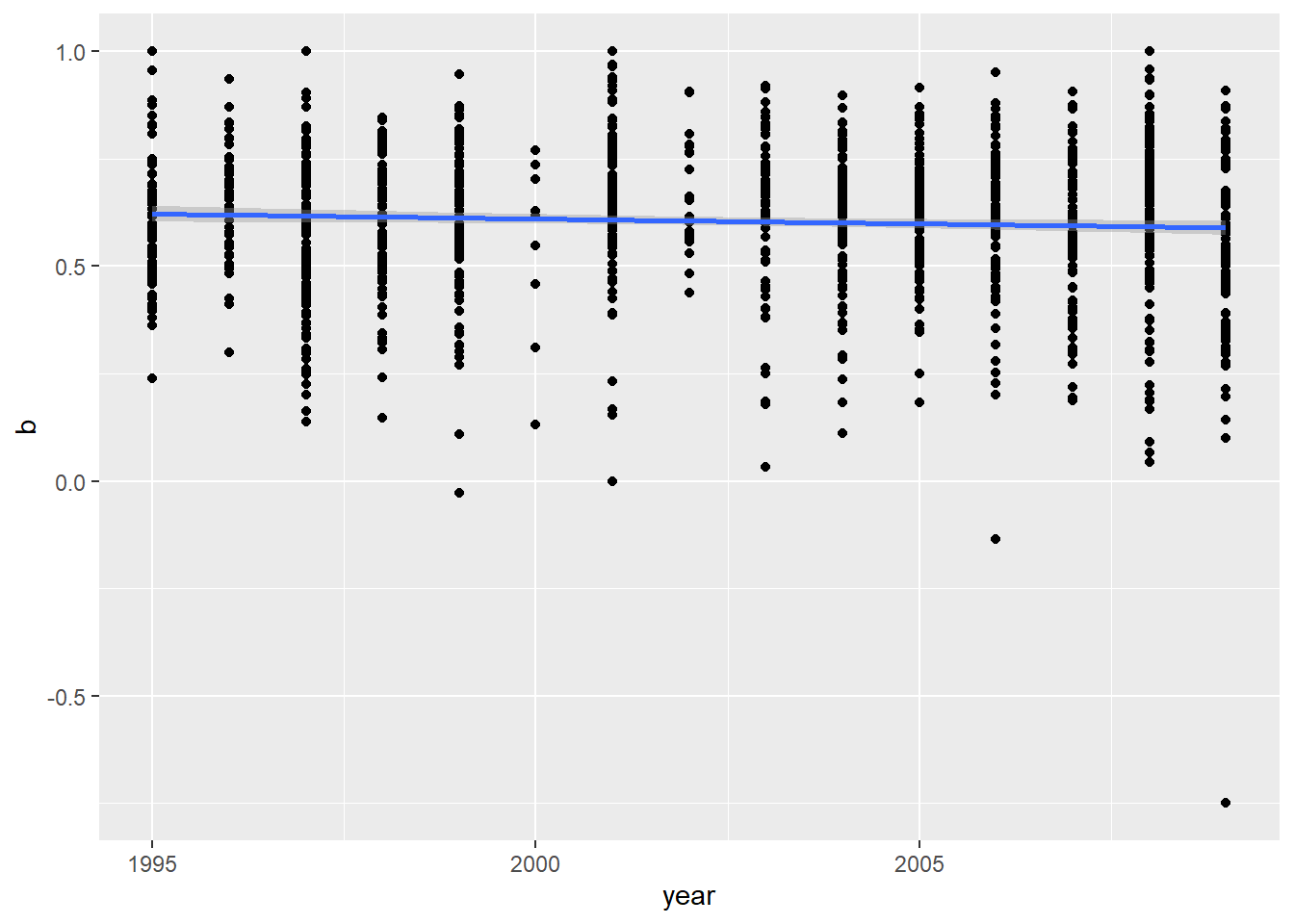
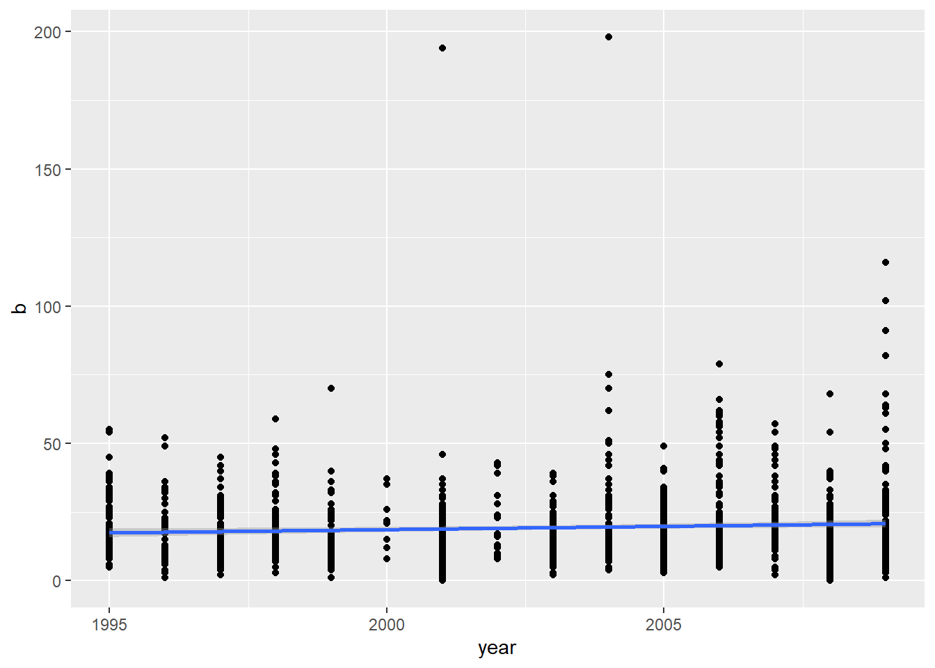
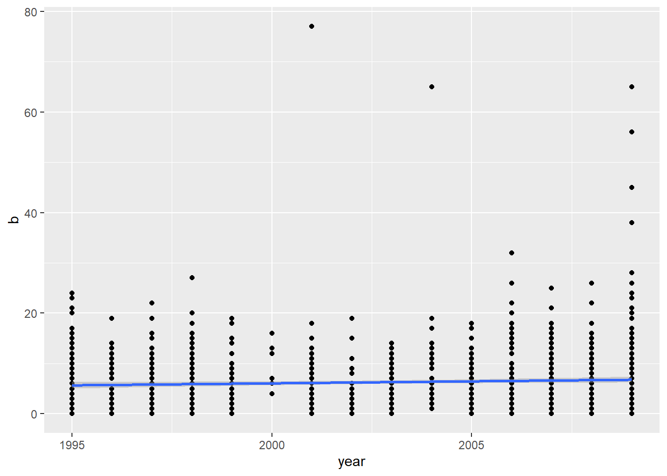
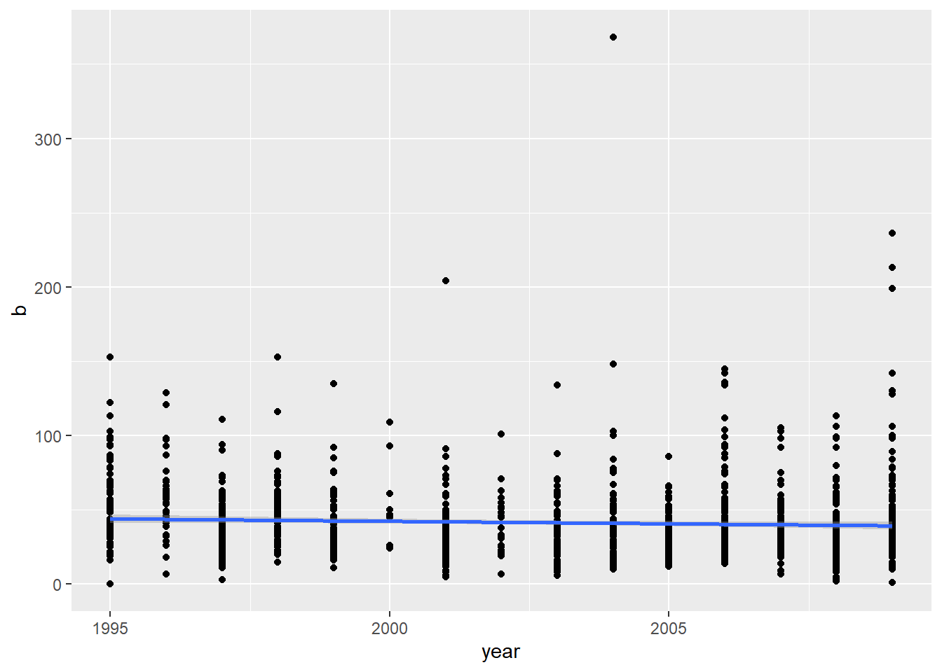
Then, I wanted to regress year on these emotions and polarity, just to see how much variance was explained by time.

Code

reg.emo <- function(b){
 emomodel <- lm(b ~ year, data = df_nrc_meta)

 emoplot <- ggplot(data = df_nrc_meta, aes(x = year, y = b)) +
   geom_point() +
   geom_smooth(method = 'lm', formula = y ~ x)
 
 print(summary(emomodel))
 emoplot
   
}

reg.emo(df_nrc_meta$polarity)

Call:
lm(formula = b ~ year, data = df_nrc_meta)

Residuals:
     Min       1Q   Median       3Q      Max 
-1.33986 -0.09879  0.01559  0.11537  0.40787 

Coefficients:
             Estimate Std. Error t value Pr(>|t|)  
(Intercept)  5.154781   2.136663   2.413   0.0160 *
year        -0.002272   0.001067  -2.130   0.0334 *
---
Signif. codes:  0 '***' 0.001 '**' 0.01 '*' 0.05 '.' 0.1 ' ' 1

Residual standard error: 0.1722 on 1258 degrees of freedom
Multiple R-squared:  0.003592,  Adjusted R-squared:  0.0028 
F-statistic: 4.536 on 1 and 1258 DF,  p-value: 0.03339

Code

reg.emo(df_nrc_meta$fear)

Call:
lm(formula = b ~ year, data = df_nrc_meta)

Residuals:
    Min      1Q  Median      3Q     Max 
-20.557  -8.419  -2.869   5.056 178.394 

Coefficients:
              Estimate Std. Error t value Pr(>|t|)   
(Intercept) -456.40293  179.06208  -2.549  0.01093 * 
year           0.23753    0.08941   2.657  0.00799 **
---
Signif. codes:  0 '***' 0.001 '**' 0.01 '*' 0.05 '.' 0.1 ' ' 1

Residual standard error: 14.43 on 1258 degrees of freedom
Multiple R-squared:  0.005578,  Adjusted R-squared:  0.004788 
F-statistic: 7.057 on 1 and 1258 DF,  p-value: 0.007995

Code

reg.emo(df_nrc_meta$anger)

Call:
lm(formula = b ~ year, data = df_nrc_meta)

Residuals:
   Min     1Q Median     3Q    Max 
-6.788 -3.709 -1.630  2.163 70.846 

Coefficients:
              Estimate Std. Error t value Pr(>|t|)  
(Intercept) -152.52334   75.79006  -2.012   0.0444 *
year           0.07930    0.03785   2.095   0.0363 *
---
Signif. codes:  0 '***' 0.001 '**' 0.01 '*' 0.05 '.' 0.1 ' ' 1

Residual standard error: 6.108 on 1258 degrees of freedom
Multiple R-squared:  0.003478,  Adjusted R-squared:  0.002686 
F-statistic:  4.39 on 1 and 1258 DF,  p-value: 0.03634

Code

reg.emo(df_nrc_meta$trust)

Call:
lm(formula = b ~ year, data = df_nrc_meta)

Residuals:
   Min     1Q Median     3Q    Max 
-44.08 -15.41  -5.07   7.93 326.93 

Coefficients:
            Estimate Std. Error t value Pr(>|t|)  
(Intercept) 711.1900   321.6387   2.211   0.0272 *
year         -0.3344     0.1606  -2.082   0.0375 *
---
Signif. codes:  0 '***' 0.001 '**' 0.01 '*' 0.05 '.' 0.1 ' ' 1

Residual standard error: 25.92 on 1258 degrees of freedom
Multiple R-squared:  0.003434,  Adjusted R-squared:  0.002642 
F-statistic: 4.335 on 1 and 1258 DF,  p-value: 0.03754

The relationships certainly look small, even if they were significant. For each dependent variable, year explained less than 1% of the variance.

Next, I followed the same procedure examining climate risk in relation to outcomes

Code

cor.emo.cri <- function(b){
  cor.test(df_nrc_meta$CRI, b, method = "pearson")
}

cor.emo.cri(df_nrc_meta$anger)

    Pearson's product-moment correlation

data:  df_nrc_meta$CRI and b
t = -1.057, df = 905, p-value = 0.2908
alternative hypothesis: true correlation is not equal to 0
95 percent confidence interval:
 -0.09998097  0.03004969
sample estimates:
        cor 
-0.03511425 

Code

cor.emo.cri(df_nrc_meta$anticipation)

    Pearson's product-moment correlation

data:  df_nrc_meta$CRI and b
t = -1.0676, df = 905, p-value = 0.286
alternative hypothesis: true correlation is not equal to 0
95 percent confidence interval:
 -0.10033077  0.02969666
sample estimates:
        cor 
-0.03546715 

Code

cor.emo.cri(df_nrc_meta$sadness)

    Pearson's product-moment correlation

data:  df_nrc_meta$CRI and b
t = -1.6627, df = 905, p-value = 0.09672
alternative hypothesis: true correlation is not equal to 0
95 percent confidence interval:
 -0.119850415  0.009945277
sample estimates:
       cor 
-0.0551857 

Code

cor.emo.cri(df_nrc_meta$disgust)

    Pearson's product-moment correlation

data:  df_nrc_meta$CRI and b
t = -1.3299, df = 905, p-value = 0.1839
alternative hypothesis: true correlation is not equal to 0
95 percent confidence interval:
 -0.10894555  0.02099211
sample estimates:
        cor 
-0.04416349 

Code

cor.emo.cri(df_nrc_meta$trust)

    Pearson's product-moment correlation

data:  df_nrc_meta$CRI and b
t = -1.5948, df = 905, p-value = 0.1111
alternative hypothesis: true correlation is not equal to 0
95 percent confidence interval:
 -0.11762957  0.01219761
sample estimates:
        cor 
-0.05293968 

Code

cor.emo.cri(df_nrc_meta$surprise)

    Pearson's product-moment correlation

data:  df_nrc_meta$CRI and b
t = -0.51025, df = 905, p-value = 0.61
alternative hypothesis: true correlation is not equal to 0
95 percent confidence interval:
 -0.08196365  0.04818957
sample estimates:
        cor 
-0.01695888 

Code

cor.emo.cri(df_nrc_meta$joy)

    Pearson's product-moment correlation

data:  df_nrc_meta$CRI and b
t = -1.687, df = 905, p-value = 0.09194
alternative hypothesis: true correlation is not equal to 0
95 percent confidence interval:
 -0.120645871  0.009138223
sample estimates:
        cor 
-0.05599034 

Code

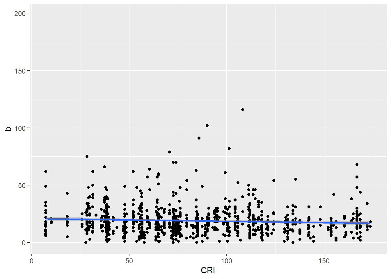
cor.emo.cri(df_nrc_meta$fear) #weirdly, higher CRI associated with less fearful? 

    Pearson's product-moment correlation

data:  df_nrc_meta$CRI and b
t = -2.1889, df = 905, p-value = 0.02886
alternative hypothesis: true correlation is not equal to 0
95 percent confidence interval:
 -0.13701662 -0.00750883
sample estimates:
        cor 
-0.07256861 

Code

cor.emo.cri(df_nrc_meta$negative) #significant, negative relationship...

    Pearson's product-moment correlation

data:  df_nrc_meta$CRI and b
t = -0.53941, df = 905, p-value = 0.5897
alternative hypothesis: true correlation is not equal to 0
95 percent confidence interval:
 -0.08292628  0.04722256
sample estimates:
       cor 
-0.0179278 

Code

cor.emo.cri(df_nrc_meta$positive) # significant, negative relationship...

    Pearson's product-moment correlation

data:  df_nrc_meta$CRI and b
t = -1.9938, df = 905, p-value = 0.04647
alternative hypothesis: true correlation is not equal to 0
95 percent confidence interval:
 -0.130664183 -0.001040645
sample estimates:
        cor 
-0.06613142 

Besides polarity, CRI was also significantly associated with sentiments of fear, positivity, and negativity. These relationships were not in the direction I expected. Higher CRI was associated with… -less fear -less negative sentiment -less positive sentiment

Next I looked at regressions for these.

Code

#now, regressions. 
reg.emo.cri <- function(b){
  emomodel <- lm(b ~ CRI, data = df_nrc_meta)
  
  emoplot <- ggplot(data = df_nrc_meta, aes(x = CRI, y = b)) +
    geom_point() +
    geom_smooth(method = 'lm', formula = y ~ x)
  
  print(summary(emomodel))
  emoplot
  
}

reg.emo.cri(df_nrc_meta$fear)

Call:
lm(formula = b ~ CRI, data = df_nrc_meta)

Residuals:
    Min      1Q  Median      3Q     Max 
-20.303  -7.940  -2.736   4.654  97.573 

Coefficients:
            Estimate Std. Error t value Pr(>|t|)    
(Intercept) 20.94813    0.97909  21.396   <2e-16 ***
CRI         -0.02331    0.01065  -2.189   0.0289 *  
---
Signif. codes:  0 '***' 0.001 '**' 0.01 '*' 0.05 '.' 0.1 ' ' 1

Residual standard error: 12.96 on 905 degrees of freedom
  (353 observations deleted due to missingness)
Multiple R-squared:  0.005266,  Adjusted R-squared:  0.004167 
F-statistic: 4.791 on 1 and 905 DF,  p-value: 0.02886

Warning: Removed 353 rows containing non-finite values (stat_smooth).

Warning: Removed 353 rows containing missing values (geom_point).

Code

reg.emo.cri(df_nrc_meta$negative)

Call:
lm(formula = b ~ CRI, data = df_nrc_meta)

Residuals:
    Min      1Q  Median      3Q     Max 
-17.595  -8.321  -2.952   4.631 133.876 

Coefficients:
            Estimate Std. Error t value Pr(>|t|)    
(Intercept) 17.75657    0.99718  17.807   <2e-16 ***
CRI         -0.00585    0.01085  -0.539     0.59    
---
Signif. codes:  0 '***' 0.001 '**' 0.01 '*' 0.05 '.' 0.1 ' ' 1

Residual standard error: 13.2 on 905 degrees of freedom
  (353 observations deleted due to missingness)
Multiple R-squared:  0.0003214, Adjusted R-squared:  -0.0007832 
F-statistic: 0.291 on 1 and 905 DF,  p-value: 0.5897

Warning: Removed 353 rows containing non-finite values (stat_smooth).
Removed 353 rows containing missing values (geom_point).

Code

reg.emo.cri(df_nrc_meta$positive)

Call:
lm(formula = b ~ CRI, data = df_nrc_meta)

Residuals:
   Min     1Q Median     3Q    Max 
-65.98 -23.60  -6.73  13.84 356.67 

Coefficients:
            Estimate Std. Error t value Pr(>|t|)    
(Intercept) 70.95827    2.88129  24.627   <2e-16 ***
CRI         -0.06248    0.03134  -1.994   0.0465 *  
---
Signif. codes:  0 '***' 0.001 '**' 0.01 '*' 0.05 '.' 0.1 ' ' 1

Residual standard error: 38.14 on 905 degrees of freedom
  (353 observations deleted due to missingness)
Multiple R-squared:  0.004373,  Adjusted R-squared:  0.003273 
F-statistic: 3.975 on 1 and 905 DF,  p-value: 0.04647

Warning: Removed 353 rows containing non-finite values (stat_smooth).
Removed 353 rows containing missing values (geom_point).

Code

reg.emo.cri(df_nrc_meta$polarity)

Call:
lm(formula = b ~ CRI, data = df_nrc_meta)

Residuals:
     Min       1Q   Median       3Q      Max 
-1.32361 -0.10122  0.01771  0.11136  0.41906 

Coefficients:
              Estimate Std. Error t value Pr(>|t|)    
(Intercept)  0.6182749  0.0128103   48.26   <2e-16 ***
CRI         -0.0002786  0.0001393   -2.00   0.0458 *  
---
Signif. codes:  0 '***' 0.001 '**' 0.01 '*' 0.05 '.' 0.1 ' ' 1

Residual standard error: 0.1696 on 905 degrees of freedom
  (353 observations deleted due to missingness)
Multiple R-squared:  0.004399,  Adjusted R-squared:  0.003299 
F-statistic: 3.998 on 1 and 905 DF,  p-value: 0.04584

Warning: Removed 353 rows containing non-finite values (stat_smooth).
Removed 353 rows containing missing values (geom_point).

Again, the relationships though significant were very small, with tiny effect sizes. I will think more about whether or not sentiment analysis is useful to me in this context…I also only looked at results from using one dictionary. In the future, I might see how/whether using different dictionaries might impact my results.

For the next step in my project, I am interested in testing out some unsupervised methods. Topic modeling might help me to identify interesting things.