Blog 3- Semantic Network Analysis

Code

knitr::opts_chunk$set(echo = TRUE, warning = FALSE)

Code

library(readr)
library(dplyr)

Attaching package: 'dplyr'

The following objects are masked from 'package:stats':

    filter, lag

The following objects are masked from 'package:base':

    intersect, setdiff, setequal, union

Code

library(quanteda)

Package version: 3.2.3
Unicode version: 13.0
ICU version: 69.1

Parallel computing: 8 of 8 threads used.

See https://quanteda.io for tutorials and examples.

Code

library(quanteda.textstats)
library(quanteda.textplots)
library(ggplot2)
library(DT)
library(tm)

Loading required package: NLP

Attaching package: 'NLP'

The following object is masked from 'package:ggplot2':

    annotate

The following objects are masked from 'package:quanteda':

    meta, meta<-

Attaching package: 'tm'

The following object is masked from 'package:quanteda':

    stopwords

Code

library(stringr)

This 3rd Blog uses text representation concepts from week 6. Using tweet replies as corpus, I will apply document-feature matrix and term-co-occurence matrix to better undersatnd the relationships of the texts. I will also apply TF-IDF: Term Frequency-Inverse Document Frequency to rank the words by frequency. Data visualization of the semantic network to understand what words co-occur with one another.

Code

# Read in data

IRA<- read_csv("IRA_med.csv")

New names:
Rows: 9497 Columns: 79
── Column specification
──────────────────────────────────────────────────────── Delimiter: "," chr
(34): edit_history_tweet_ids, text, lang, source, reply_settings, entit... dbl
(18): id, conversation_id, referenced_tweets.replied_to.id, referenced_... lgl
(23): referenced_tweets.retweeted.id, edit_controls.is_edit_eligible, r... dttm
(4): edit_controls.editable_until, created_at, author.created_at, __tw...
ℹ Use `spec()` to retrieve the full column specification for this data. ℹ
Specify the column types or set `show_col_types = FALSE` to quiet this message.
• `` -> `...79`

Code

#remove @twitter handles
IRA$text <- gsub("@[[:alpha:]]*","", IRA$text) #remove Twitter handles

Code

IRA_corpus <- corpus(IRA,text_field = "text")   

#tokenize and stemming

Code

IRA_tokens <- tokens(IRA_corpus)
IRA_tokens <- tokens_wordstem(IRA_tokens)

Locate keywords in text

I played around with this and compared results from keywords :“inflation”, “pharma”, and “price”.

Code

IRA_kw <- kwic(IRA_tokens, pattern =  "price*", window = 3,
  valuetype = c("glob", "regex", "fixed"),
  separator = " ",
  case_insensitive = TRUE,
  index = NULL) 
head(IRA_kw, 5) 

Keyword-in-context with 5 matches.                                                              
   [text2, 10]    see those cheap | price | on my prescript   
  [text22, 16]       the US allow | price | goug. That        
   [text49, 6]   that these lower | price | aren't lower price
   [text49, 9] price aren't lower | price | ?? You'r          
 [text117, 18]          HIGH. Gas | price | in CA are         

#TF-IDF rank words by term frequency

Code

IRA_dfm <- tokens(IRA_corpus, remove_punct = TRUE, remove_numbers = TRUE, remove_symbols = TRUE, remove_url=TRUE) %>%  
  tokens_remove (stopwords("en")) %>%
  dfm()
topfeatures(IRA_dfm) 

      big inflation    pharma         n    people     biden      lost  american 
     1307      1225      1174       873       822       485       467       456 
      act      will 
      438       433 

#rank words by TF-IDF

Code

IRA_dfm <- dfm_tfidf(IRA_dfm) 
topfeatures(IRA_dfm) 

inflation       big    pharma         n    people     biden      lost  american 
1199.1418 1193.4589 1108.9193 1058.6552  901.0779  648.4959  618.0324  611.9988 
     will       act 
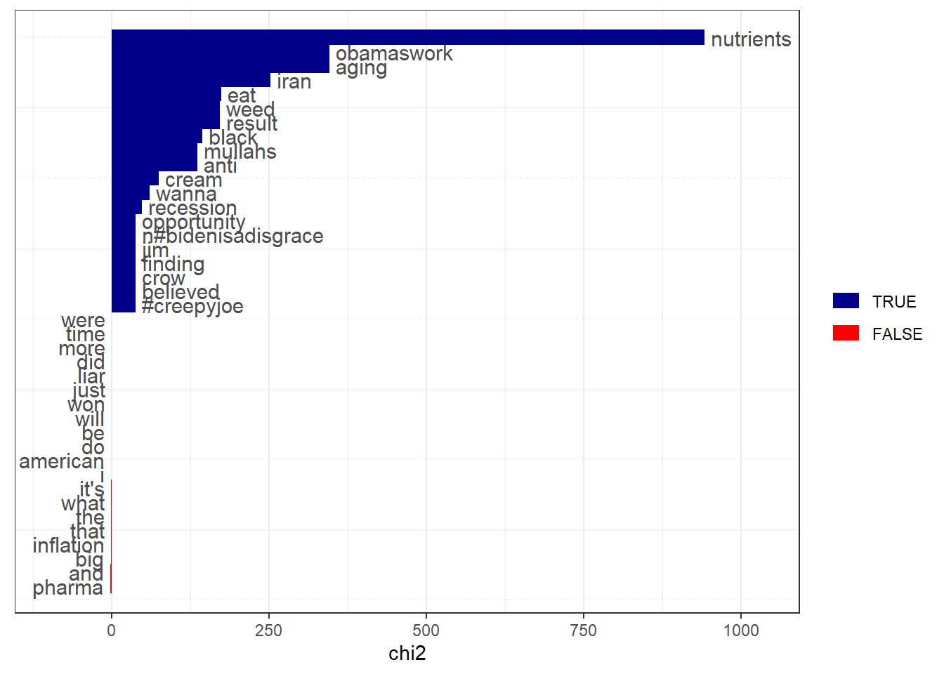
 609.2498  599.6485 

#Keyness analysis as an alternative to tf-idf I grouped the responses as based on possible sensitivity of the tweet replies. The possibly sensitive =TRUE replies “keywords” compared to the associations and a reference group of possible_sensitive= FALSE group replies,

Code

IRA_dfm <- tokens(IRA_corpus, remove_punct = TRUE, remove_numbers = TRUE, remove_symbols = TRUE, remove_url=TRUE) %>%
  dfm() %>%
  dfm_group(groups = possibly_sensitive)  

IRAkey <- textstat_keyness(IRA_dfm, target = "TRUE")
textplot_keyness(IRAkey,
  show_reference = TRUE,
  show_legend = TRUE,
  n = 20L,
  min_count = 2L,
  margin = 0.05,
  color = c("darkblue", "red"),
  labelcolor = "gray30",
  labelsize = 4,
  font = NULL
)

DFM that contains hashtags

Code

IRAtag_dfm <- dfm_select(IRA_dfm, pattern = "#*")
IRAtoptag <- names(topfeatures(IRA_dfm, 50)) 
head(IRAtoptag)

[1] "the" "you" "to"  "and" "a"   "is" 

#Feature-occurrence matrix of hashtags

Code

IRAtag_fcm <- fcm(IRA_dfm)
head(IRAtag_fcm)

Feature co-occurrence matrix of: 6 by 11,231 features.
        features
features     so   when     do      i    get      to    see  those cheap prices
    so   119805 172481 222460 433651 143080 1315660  87710  55862  4900 133770
    when      0  61776 159808 311521 102784  945130  63008  40130  3520  96096
    do        0      0 102831 401790 132568 1218990  81266  51756  4540 123942
    i         0      0      0 391170 258420 2376235 158415 100892  8850 241605
    get       0      0      0      0  42486  784020  52268  33288  2920  79716
    to        0      0      0      0      0 3603315 480615 306110 26850 733005
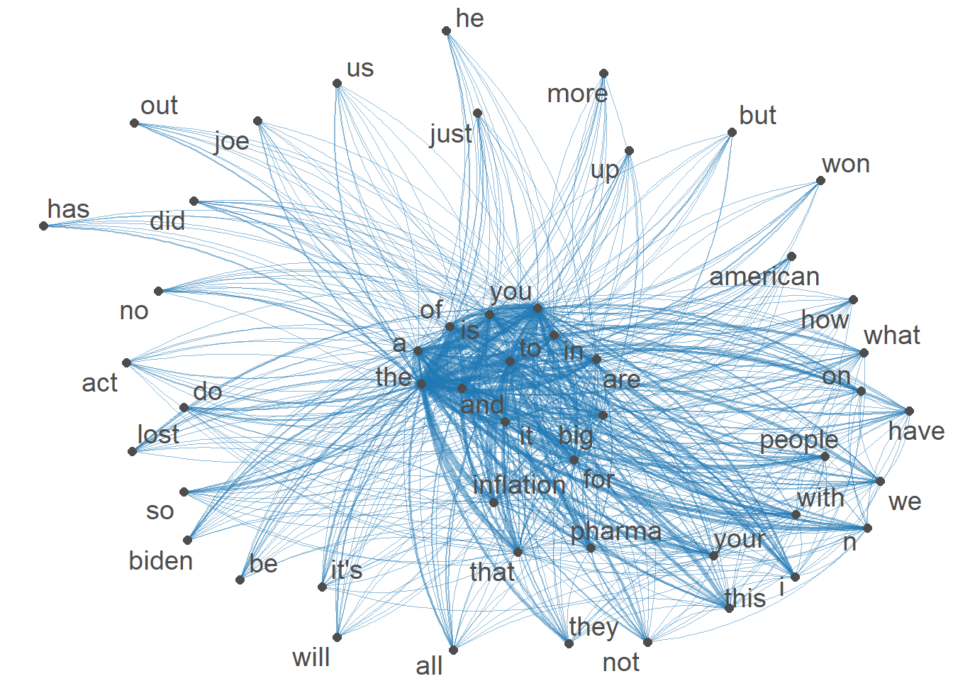
[ reached max_nfeat ... 11,221 more features ]

#Visualization of semantic network based on hashtag co-occurrence

Code

IRAtopgat_fcm <- fcm_select(IRAtag_fcm, pattern = IRAtoptag)
textplot_network(IRAtopgat_fcm, min_freq = 0.5,
  omit_isolated = TRUE,
  edge_color = "#1F78B4",
  edge_alpha = 0.5,
  edge_size = 2,
  vertex_color = "#4D4D4D",
  vertex_size = 2,
  vertex_labelcolor = NULL,
  vertex_labelfont = NULL,
  vertex_labelsize = 5,
  offset = NULL)