Blog 6-Focus on Sentiment Analysis of MA Gubernatorial Candidate Tweet Replies

Blog 6

Twitter Replies

Twarc2

Rhowena Vespa

Massachusetts Gubernatorial Elections

Healey

Diehl

Sentiment Analysis

Author

Rhowena Vespa

Published

November 30, 2022

Code

knitr::opts_chunk$set(echo = TRUE, warning = FALSE, StringsAsFActors= FALSE)

Update: For the final blog post, I have decided to focus on Sentiment Analysis and any correlation to Twitter Data. This post builds on previous blog posts and a more detailed analysis on sentiments from Twitter Data

This project analyzes Twitter engagement of specific Massachusetts Governor Candidates namely Maura Healey and Geoff Diehl.

CORPUS: Extracted twitter replies (Oct 29 to Nov 4) from all of Healey and Diehl’s tweets. The replies looks into how these candidates engages other twitter users by generating a response to their original tweet or retweet.

The replies are then cleaned and pre-processed.

Analysis:

    Initial Data visualization (word cloud)
    TF-IDF
    Semantic Network Analysis
    Sentiment Analysis + Polarity

LOAD PACKAGES

Code

library(readr)
library(dplyr)


Attaching package: 'dplyr'

The following objects are masked from 'package:stats':

    filter, lag

The following objects are masked from 'package:base':

    intersect, setdiff, setequal, union

Code

library(quanteda)

Package version: 3.2.3
Unicode version: 13.0
ICU version: 69.1

Parallel computing: 8 of 8 threads used.

See https://quanteda.io for tutorials and examples.

Code

library(quanteda.textstats)
library(quanteda.textplots)
library(ggplot2)
library(DT)
library(tm)

Loading required package: NLP


Attaching package: 'NLP'

The following object is masked from 'package:ggplot2':

    annotate

The following objects are masked from 'package:quanteda':

    meta, meta<-


Attaching package: 'tm'

The following object is masked from 'package:quanteda':

    stopwords

Code

library(stringr)
library(tidyverse)

── Attaching packages
───────────────────────────────────────
tidyverse 1.3.2 ──

✔ tibble  3.1.8     ✔ purrr   0.3.5
✔ tidyr   1.2.1     ✔ forcats 0.5.2
── Conflicts ────────────────────────────────────────── tidyverse_conflicts() ──
✖ NLP::annotate() masks ggplot2::annotate()
✖ dplyr::filter() masks stats::filter()
✖ dplyr::lag()    masks stats::lag()

Code

library(tidytext)
library(plyr)

------------------------------------------------------------------------------
You have loaded plyr after dplyr - this is likely to cause problems.
If you need functions from both plyr and dplyr, please load plyr first, then dplyr:
library(plyr); library(dplyr)
------------------------------------------------------------------------------

Attaching package: 'plyr'

The following object is masked from 'package:purrr':

    compact

The following objects are masked from 'package:dplyr':

    arrange, count, desc, failwith, id, mutate, rename, summarise,
    summarize

Code

library(tidyverse)
library(quanteda.textmodels)
library(devtools)

Loading required package: usethis

Code

library(caret)

Loading required package: lattice

Attaching package: 'caret'

The following object is masked from 'package:purrr':

    lift

Code

library(e1071)
library(quanteda.dictionaries)
#library(devtools)
#devtools::install_github("kbenoit/quanteda.dictionaries")
library(quanteda.dictionaries)
library(syuzhet) 
#remotes::install_github("quanteda/quanteda.sentiment")
library(quanteda.sentiment)


Attaching package: 'quanteda.sentiment'

The following object is masked from 'package:quanteda':

    data_dictionary_LSD2015

Code

library(lubridate)


Attaching package: 'lubridate'

The following objects are masked from 'package:base':

    date, intersect, setdiff, union

Healey DATA

Load Data

Code

Healy <- read_csv("Healy.csv")

Rows: 1900 Columns: 79
── Column specification ────────────────────────────────────────────────────────
Delimiter: ","
chr  (33): edit_history_tweet_ids, text, lang, source, reply_settings, entit...
dbl  (18): id, conversation_id, referenced_tweets.replied_to.id, referenced_...
lgl  (24): referenced_tweets.retweeted.id, edit_controls.is_edit_eligible, r...
dttm  (4): edit_controls.editable_until, created_at, author.created_at, __tw...

ℹ Use `spec()` to retrieve the full column specification for this data.
ℹ Specify the column types or set `show_col_types = FALSE` to quiet this message.

Code

Healy$text <- gsub("@[[:alpha:]]*","", Healy$text) #remove Twitter handles
Healy$text <- gsub("&amp", "", Healy$text)
Healy$text <- gsub("healey", "", Healy$text)
Healy$text <- gsub("_", "", Healy$text)

Data Cleaning/ Preprocessing

Code

Healy_corpus <- Corpus(VectorSource(Healy$text))
Healy_corpus <- tm_map(Healy_corpus, tolower) #lowercase
Healy_corpus <- tm_map(Healy_corpus, removeWords,c("s","healey", "healy","vote", "votes","voted","Voter","maura","rt", "amp",(stopwords("english"))))
Healy_corpus <- tm_map(Healy_corpus, removePunctuation)
Healy_corpus <- tm_map(Healy_corpus, stripWhitespace)
Healy_corpus <- tm_map(Healy_corpus, removeNumbers)

Tokenize and stemming

Code

Healy_corpus <- corpus(Healy_corpus,text_field = "text") 
Healy_text_df <- as.data.frame(Healy_corpus)
Healy_tokens <- tokens(Healy_corpus)
Healy_tokens <- tokens_wordstem(Healy_tokens) 
print(Healy_tokens)

Tokens consisting of 1,900 documents.
text1 :
 [1] "four"       "day"        "nov"        "th"         "best"      
 [6] "pitchnnfor" "starter"    "abort"      "fulli"      "protect"   
[11] "ma"         "chang"     
[ ... and 14 more ]

text2 :
 [1] "reproduct"  "freedom"    "protect"    "ma"         "sent"      
 [6] "back"       "state"      "…"          "belong"     "ag"        
[11] "understand"

text3 :
 [1] "serious"    "state"      "'"          "follow"     "scienc"    
 [6] "'"          "w"          "experiment" "drug"       "young"     
[11] "femal"      "'"         
[ ... and 12 more ]

text4 :
[1] "preserv"   "democraci" "come"      "man"      

text5 :
[1] "protect" "kid"     "mean"    "vote"   

text6 :
 [1] "like"            "serious"         "guy"             "republican"     
 [5] "fix"             "anyth"           "claim"           "abl"            
 [9] "just"            "gonna"           "pull"            "sociallyconserv"
[ ... and 10 more ]

[ reached max_ndoc ... 1,894 more documents ]

Code

dfm(Healy_tokens)

Document-feature matrix of: 1,900 documents, 3,683 features (99.79% sparse) and 0 docvars.
       features
docs    four day nov th best pitchnnfor starter abort fulli protect
  text1    1   1   1  1    1          1       1     1     1       1
  text2    0   0   0  0    0          0       0     0     0       1
  text3    0   0   0  0    0          0       0     0     0       2
  text4    0   0   0  0    0          0       0     0     0       0
  text5    0   0   0  0    0          0       0     0     0       1
  text6    0   0   0  0    0          0       0     0     0       0
[ reached max_ndoc ... 1,894 more documents, reached max_nfeat ... 3,673 more features ]

Create dfm

Code

# create a full dfm for comparison---use this to append to polarity
Healy_Dfm <- tokens(Healy_tokens,
                  remove_punct = TRUE,
                  remove_symbols = TRUE,
                  remove_numbers = TRUE,
                  remove_url = TRUE,
                  split_hyphens = FALSE,
                  split_tags = FALSE,
                  include_docvars = TRUE) %>%
  tokens_tolower() %>%
  dfm(remove = stopwords('english')) %>%
  dfm_trim(min_termfreq = 10, verbose = FALSE) %>%
  dfm()

TF-IDF

Code

topfeatures(Healy_Dfm)

    will       go    peopl    state     like democrat    right     just 
     124      123      117      114      100       96       93       89 
   elect     vote 
      89       88

Code

Healy_tf_dfm <- dfm_tfidf(Healy_Dfm, force = TRUE) #create a new DFM by tf-idf scores
topfeatures(Healy_tf_dfm) ## this shows top words by tf-idf

    will       go    state    peopl     like democrat    right    elect 
152.9454 151.2329 145.2853 145.2353 132.4511 127.6189 125.0157 121.0111 
    vote     just 
120.5836 119.1919

Code

# convert corpus to dfm using the dictionary---use to append ???
HealyDfm_nrc <- tokens(Healy_tokens,
                     remove_punct = TRUE,
                     remove_symbols = TRUE,
                     remove_numbers = TRUE,
                     remove_url = TRUE,
                     split_tags = FALSE,
                     split_hyphens = FALSE,
                     include_docvars = TRUE) %>%
  tokens_tolower() %>%
  dfm(remove = stopwords('english')) %>%
  dfm_trim(min_termfreq = 10, verbose = FALSE) %>%
  dfm() %>%
  dfm_lookup(data_dictionary_NRC)

Word Cloud

Code

library(RColorBrewer)
textplot_wordcloud(Healy_Dfm, scale=c(5,1), max.words=40, random.order=FALSE, rot.per=0.35, use.r.layout=FALSE, colors=brewer.pal(8, "Dark2"))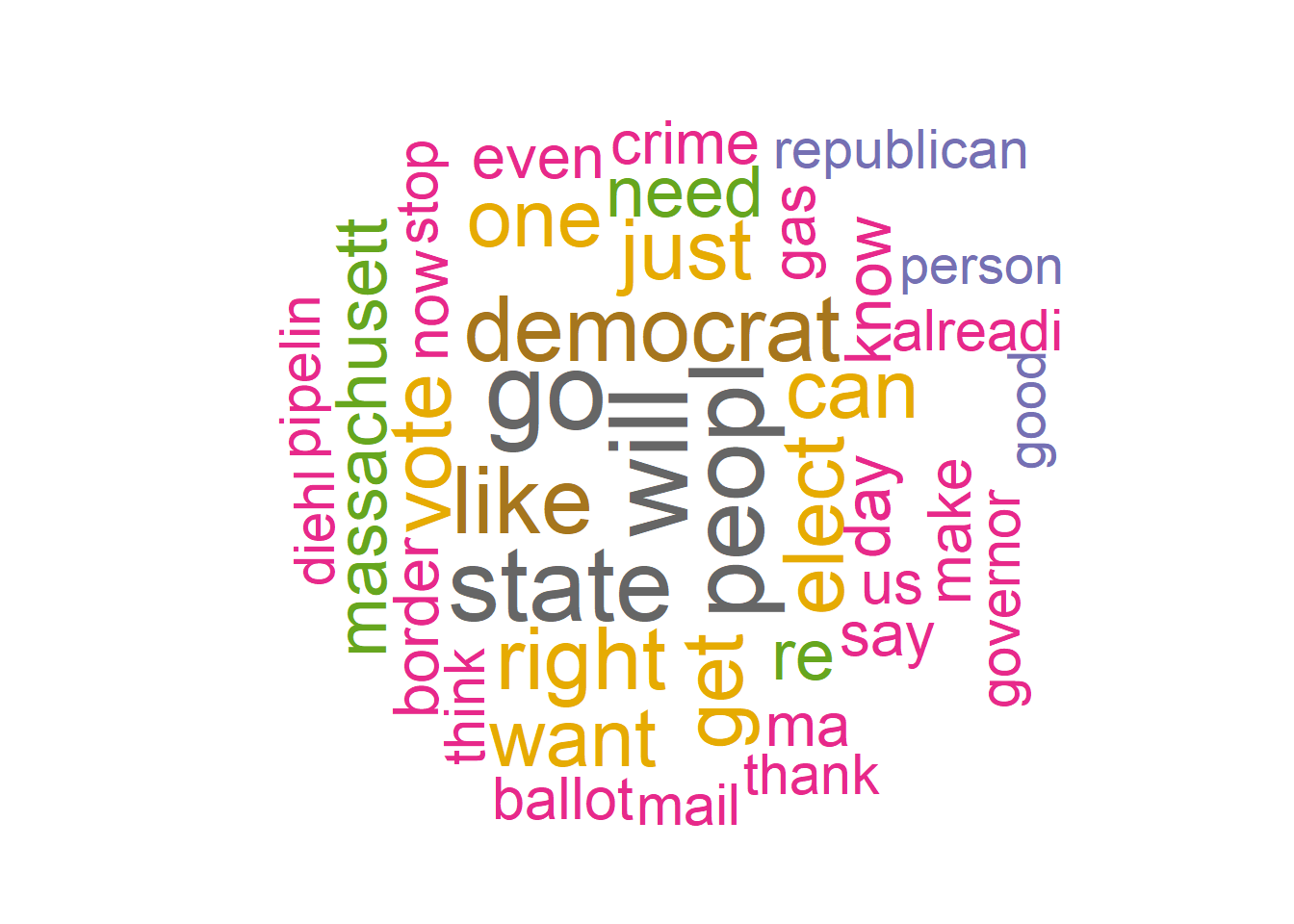

Feature-Occurence Matrix

Code

# DFM that contains hashtags 
Healytag_dfm <- dfm_select(Healy_Dfm, pattern = "#*")
Healytoptag <- names(topfeatures(Healy_Dfm, 30)) 
head(Healytoptag)

[1] "will"     "go"       "peopl"    "state"    "like"     "democrat"

Code

Healytag_fcm <- fcm(Healy_Dfm, context = "document", tri = FALSE)
head(Healytag_fcm)

Feature co-occurrence matrix of: 6 by 334 features.
         features
features  day th best abort protect ma chang two just anyth
  day       3  1    2     1       1  3     1   1    9     1
  th        1  0    1     2       1  2     1   1    1     1
  best      2  1    0     1       2  2     1   1    1     1
  abort     1  2    1     0       1  2     1   1    1     1
  protect   1  1    2     1       4  3     1   1    2     1
  ma        3  2    2     2       3  1     2   3    5     2
[ reached max_nfeat ... 324 more features ]

Semantic Network Visualization

Code

#Visualization of semantic network based on hashtag co-occurrence
Healytopgat_fcm <- fcm_select(Healytag_fcm, pattern = Healytoptag)
textplot_network(Healytopgat_fcm, min_freq = 1.2,
                 omit_isolated = TRUE,
                 edge_color = "#1F78B4",
                 edge_alpha = 0.5,
                 edge_size = 2,
                 vertex_color = "black",
                 vertex_size = 2,
                 vertex_labelcolor = NULL,
                 vertex_labelfont = NULL,
                 vertex_labelsize = 8,
                 offset = NULL)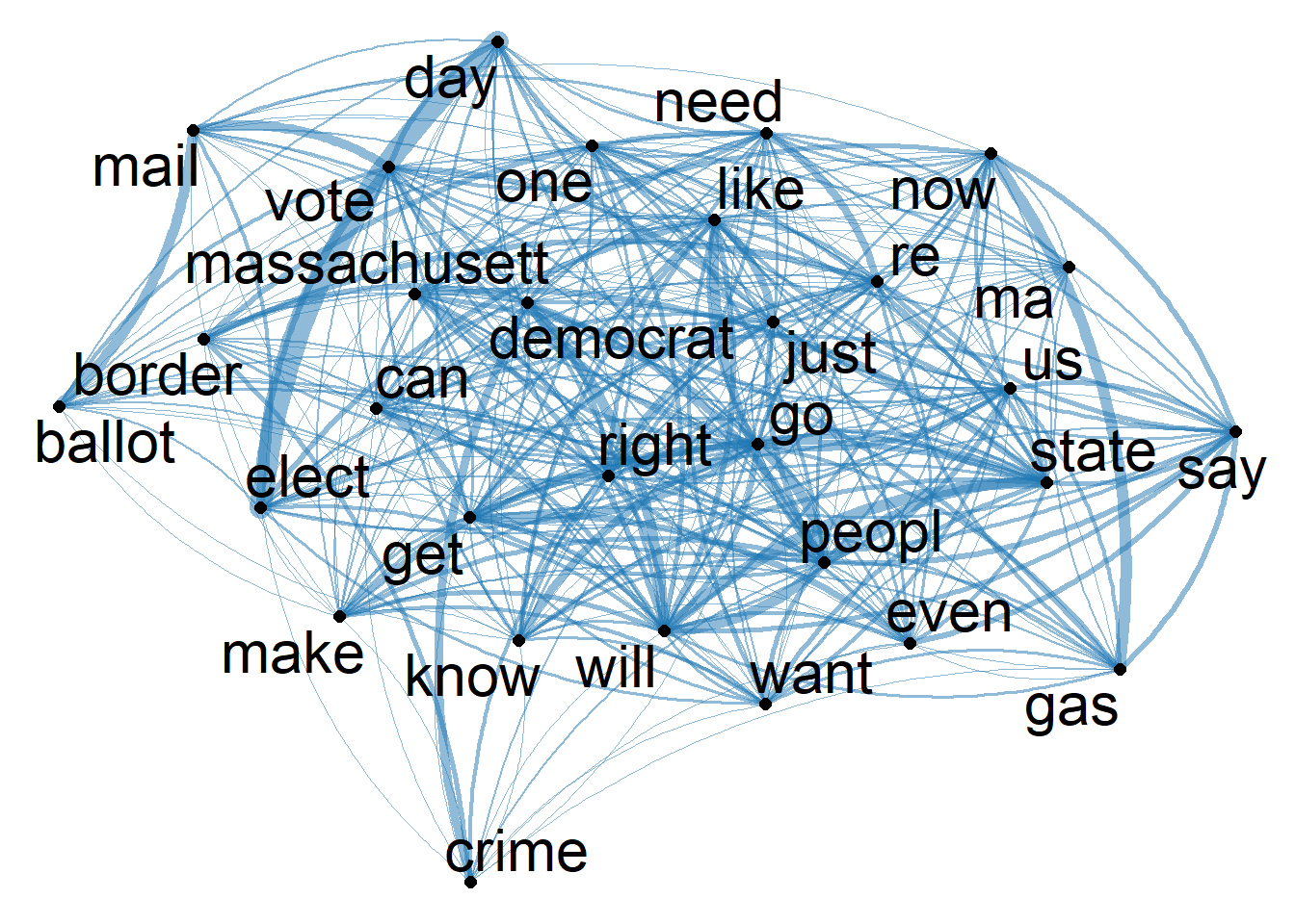

Code

textplot_network(Healytopgat_fcm, vertex_labelsize = 3 * rowSums(Healytopgat_fcm)/min(rowSums(Healytopgat_fcm)))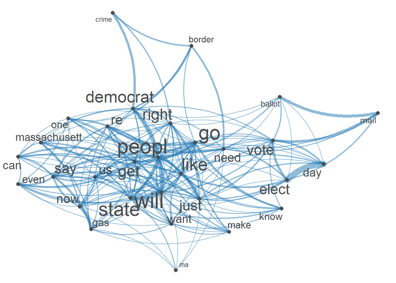

Code

H_csv <- as.data.frame((cbind(Healy,Healy_text_df)))
write_csv(H_csv,"H_csv")

NRC Sentiment Analysis

Code

H_Sentiment <- get_nrc_sentiment(H_csv$Healy_corpus)

Code

H_all_senti <- cbind(H_Sentiment, H_csv)  #Combine sentiment ratings to create a new data frame

Code

summary(H_Sentiment)

     anger         anticipation       disgust            fear       
 Min.   :0.0000   Min.   :0.0000   Min.   :0.0000   Min.   :0.0000  
 1st Qu.:0.0000   1st Qu.:0.0000   1st Qu.:0.0000   1st Qu.:0.0000  
 Median :0.0000   Median :0.0000   Median :0.0000   Median :0.0000  
 Mean   :0.2911   Mean   :0.3284   Mean   :0.2158   Mean   :0.3342  
 3rd Qu.:0.0000   3rd Qu.:1.0000   3rd Qu.:0.0000   3rd Qu.:0.0000  
 Max.   :5.0000   Max.   :5.0000   Max.   :4.0000   Max.   :4.0000  
      joy            sadness          surprise        trust       
 Min.   :0.0000   Min.   :0.0000   Min.   :0.00   Min.   :0.0000  
 1st Qu.:0.0000   1st Qu.:0.0000   1st Qu.:0.00   1st Qu.:0.0000  
 Median :0.0000   Median :0.0000   Median :0.00   Median :0.0000  
 Mean   :0.2511   Mean   :0.2547   Mean   :0.16   Mean   :0.4489  
 3rd Qu.:0.0000   3rd Qu.:0.0000   3rd Qu.:0.00   3rd Qu.:1.0000  
 Max.   :4.0000   Max.   :4.0000   Max.   :3.00   Max.   :7.0000  
    negative         positive     
 Min.   :0.0000   Min.   :0.0000  
 1st Qu.:0.0000   1st Qu.:0.0000  
 Median :0.0000   Median :0.0000  
 Mean   :0.5837   Mean   :0.7026  
 3rd Qu.:1.0000   3rd Qu.:1.0000  
 Max.   :6.0000   Max.   :7.0000

##POLARITY SCORES??

Code

# POLARITY

H_all_senti$polarity <- (H_all_senti$positive - H_all_senti$negative)/(H_all_senti$positive + H_all_senti$negative)

H_all_senti$polarity[(H_all_senti$positive + H_all_senti$negative) == 0] <- 0

ggplot(H_all_senti) +
  geom_histogram(aes(x=polarity)) +
  theme_bw()

`stat_bin()` using `bins = 30`. Pick better value with `binwidth`.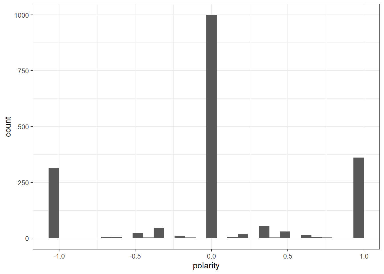

Code

datatable(H_all_senti[1:50,], options = list(pageLength = 5))

ANOTHER Sentiment Analysis NRC summary

Sentiment Analysis

Code

#convert cleaned Healy_tokens back tp corpus for sentiment analysis
Healy_corpus <- corpus(as.character(Healy_tokens))

NRC Dictionary

Code

# use liwcalike() to estimate sentiment using NRC dictionary
HealyTweetSentiment_nrc <- liwcalike(Healy_corpus, data_dictionary_NRC)
names(HealyTweetSentiment_nrc)

 [1] "docname"      "Segment"      "WPS"          "WC"           "Sixltr"      
 [6] "Dic"          "anger"        "anticipation" "disgust"      "fear"        
[11] "joy"          "negative"     "positive"     "sadness"      "surprise"    
[16] "trust"        "AllPunc"      "Period"       "Comma"        "Colon"       
[21] "SemiC"        "QMark"        "Exclam"       "Dash"         "Quote"       
[26] "Apostro"      "Parenth"      "OtherP"

Code

HealyTweetSentiment_nrc_viz <- HealyTweetSentiment_nrc %>%
  select(c("anger", "anticipation", "disgust", "fear","joy","sadness", "surprise","trust","positive","negative"))

Code

Healy_tr<-data.frame(t(HealyTweetSentiment_nrc_viz)) #transpose

Code

Healy_tr_new <- data.frame(rowSums(Healy_tr[2:1900]))
Healy_tr_mean <- data.frame(rowMeans(Healy_tr[2:1900]))#get mean of sentiment values
names(Healy_tr_new)[1] <- "Count"
Healy_tr_new <- cbind("sentiment" = rownames(Healy_tr_new), Healy_tr_new)
rownames(Healy_tr_new) <- NULL
Healy_tr_new2<-Healy_tr_new[1:8,]

Code

write_csv(Healy_tr_new2,"Healy-Sentiments")
write_csv(Healy_tr_new,"Healy-8 Sentiments")

Code

#Plot One - Count of words associated with each sentiment
quickplot(sentiment, data=Healy_tr_new2, weight=Count, geom="bar", fill=sentiment, ylab="count")+ggtitle("Emotions of REPLIES to Maura Healey Tweets")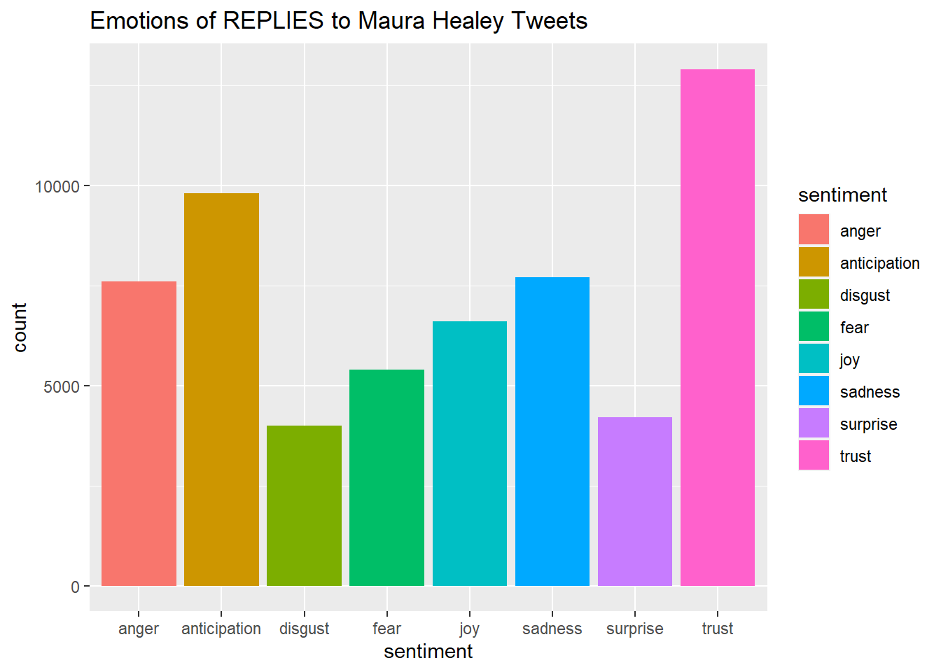

Code

names(Healy_tr_mean)[1] <- "Mean"
Healy_tr_mean <- cbind("sentiment" = rownames(Healy_tr_mean), Healy_tr_mean)
rownames(Healy_tr_mean) <- NULL
Healy_tr_mean2<-Healy_tr_mean[9:10,]
write_csv(Healy_tr_mean2,"Healy-Mean Sentiments")

Code

#Plot One - Count of words associated with each sentiment
quickplot(sentiment, data=Healy_tr_mean2, weight=Mean, geom="bar", fill=sentiment, ylab="Mean Sentiment Score")+ggtitle("Mean Sentiment Scores to Maura Healey Tweets")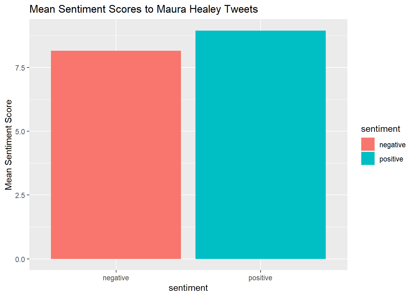

DIEHL DATA

Load Data

Code

Diehl <- read_csv("Diehl.csv")

Rows: 497 Columns: 79
── Column specification ────────────────────────────────────────────────────────
Delimiter: ","
chr  (34): edit_history_tweet_ids, text, lang, source, reply_settings, entit...
dbl  (18): id, conversation_id, referenced_tweets.replied_to.id, referenced_...
lgl  (23): referenced_tweets.retweeted.id, edit_controls.is_edit_eligible, r...
dttm  (4): edit_controls.editable_until, created_at, author.created_at, __tw...

ℹ Use `spec()` to retrieve the full column specification for this data.
ℹ Specify the column types or set `show_col_types = FALSE` to quiet this message.

Code

Diehl$text <- gsub("@[[:alpha:]]*","", Diehl$text) #remove Twitter handles
Diehl$text <- gsub("&amp", "", Diehl$text)
Diehl$text <- gsub("_", "", Diehl$text)

Data Cleaning/ Preprocessing

Code

Diehl_corpus <- Corpus(VectorSource(Diehl$text))
Diehl_corpus <- tm_map(Diehl_corpus, tolower) #lowercase
Diehl_corpus <- tm_map(Diehl_corpus, removeWords, 
                       c("s","geoff", "diehl","rt", "Vote","voter","voted", "amp"))
Diehl_corpus <- tm_map(Diehl_corpus, removeWords, 
                       stopwords("english"))
Diehl_corpus <- tm_map(Diehl_corpus, removePunctuation)
Diehl_corpus <- tm_map(Diehl_corpus, stripWhitespace)
Diehl_corpus <- tm_map(Diehl_corpus, removeNumbers)

Diehl_corpus <- corpus(Diehl_corpus,text_field = "text") 

Diehl_text_df <- as.data.frame(Diehl_corpus)

Tokenize and stemming

Code

Diehl_tokens <- tokens(Diehl_corpus)
Diehl_tokens <- tokens_wordstem(Diehl_tokens)
print(Diehl_tokens)

Tokens consisting of 497 documents.
text1 :
[1] "still"   "beat"    "fascism" "day"     "week"    "📴"     

text2 :
[1] "wear" "mask" "'"    "re"   "dumb"

text3 :
 [1] "'"       "mention" "mask"    "pay"     "compani" "can"     "charg"  
 [8] "whatev"  "want"    "follow"  "'"       "ll"     
[ ... and 10 more ]

text4 :
 [1] "argument" "gas"      "pipelin"  "energi"   "independ" "right"   
 [7] "now"      "new"      "england"  "get"      "lng"      "deliveri"
[ ... and 18 more ]

text5 :
 [1] "shit"     "u"        "dumb"     "masker"   "democrat" "still"   
 [7] "fuck"     "everyon"  "caus"     "price"    "hike"     "higher"  
[ ... and 7 more ]

text6 :
 [1] "compani"  "take"     "profit"   "loss"     "kinder"   "morgan"  
 [7] "elect"    "need"     "proof"    "energi"   "independ" "way"     
[ ... and 7 more ]

[ reached max_ndoc ... 491 more documents ]

Code

dfm(Diehl_tokens)

Document-feature matrix of: 497 documents, 1,921 features (99.49% sparse) and 0 docvars.
       features
docs    still beat fascism day week📴 wear mask ' re
  text1     1    1       1   1    1 1    0    0 0  0
  text2     0    0       0   0    0 0    1    1 1  1
  text3     0    0       0   0    0 0    0    1 2  0
  text4     0    0       0   0    0 0    0    0 0  0
  text5     1    0       0   0    0 0    0    0 0  0
  text6     0    0       0   0    0 0    0    0 0  0
[ reached max_ndoc ... 491 more documents, reached max_nfeat ... 1,911 more features ]

Create dfm

Code

# create a full dfm for comparison---use this to append to polarity
Diehl_Dfm <- tokens(Diehl_tokens,
                    remove_punct = TRUE,
                    remove_symbols = TRUE,
                    remove_numbers = TRUE,
                    remove_url = TRUE,
                    split_hyphens = FALSE,
                    split_tags = FALSE,
                    include_docvars = TRUE) %>%
  tokens_tolower() %>%
  dfm(remove = stopwords('english')) %>%
  dfm_trim(min_termfreq = 10, verbose = FALSE) %>%
  dfm()

TF-IDF

Code

topfeatures(Diehl_Dfm)

school     go   vote   like   will    get healey public   know   just 
    54     47     46     43     43     39     39     35     32     32

Code

Diehl_tf_dfm <- dfm_tfidf(Diehl_Dfm, force = TRUE) #create a new DFM by tf-idf scores
topfeatures(Diehl_tf_dfm) ## this shows top words by tf-idf

  school       go     vote     like     will      get   healey   public 
61.56291 50.43603 49.84434 46.14361 46.14361 44.46210 44.46210 43.18854 
    know     just 
39.97435 39.48667

Code

# convert corpus to dfm using the dictionary---use to append 
DiehlDfm_nrc <- tokens(Diehl_tokens,
                       remove_punct = TRUE,
                       remove_symbols = TRUE,
                       remove_numbers = TRUE,
                       remove_url = TRUE,
                       split_tags = FALSE,
                       split_hyphens = FALSE,
                       include_docvars = TRUE) %>%
  tokens_tolower() %>%
  dfm(remove = stopwords('english')) %>%
  dfm_trim(min_termfreq = 6, verbose = FALSE) %>%
  dfm() %>%
  dfm_lookup(data_dictionary_NRC)


dim(DiehlDfm_nrc)

[1] 497  10

Code

head(DiehlDfm_nrc, 10)

Document-feature matrix of: 10 documents, 10 features (66.00% sparse) and 0 docvars.
       features
docs    anger anticipation disgust fear joy negative positive sadness surprise
  text1     0            0       0    0   0        0        0       0        0
  text2     0            0       0    0   0        1        0       0        0
  text3     1            2       0    0   2        2        2       1        1
  text4     1            3       0    0   1        0        3       0        1
  text5     0            0       0    0   0        2        0       1        0
  text6     0            0       0    0   0        0        2       0        0
       features
docs    trust
  text1     0
  text2     0
  text3     2
  text4     1
  text5     0
  text6     2
[ reached max_ndoc ... 4 more documents ]

Word CLoud

Code

library(RColorBrewer)
textplot_wordcloud(Diehl_Dfm, scale=c(5,1), max.words=40, random.order=FALSE, rot.per=0.35, use.r.layout=FALSE, colors=brewer.pal(8, "Dark2"))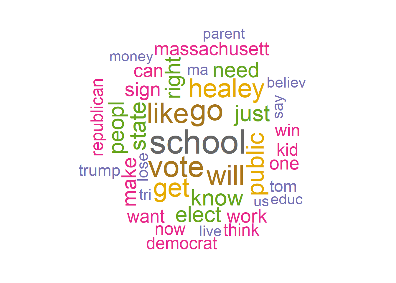

Feature-occurrence matrix

Code

Diehltag_dfm <- dfm_select(Diehl_Dfm, pattern = "#*")
Diehltoptag <- names(topfeatures(Diehl_Dfm, 30)) 
head(Diehltoptag)

[1] "school" "go"     "vote"   "like"   "will"   "get"

Code

Diehltag_fcm <- fcm(Diehl_Dfm)
head(Diehltag_fcm)

Feature co-occurrence matrix of: 6 by 74 features.
        features
features re can want see vote like gas energi right now
    re    1   0    2   0    0    1   0      1     4   0
    can   0   1    3   1    4    3   2      2     2   2
    want  0   0    4   1    2    3   0      0     4   3
    see   0   0    0   1    5    3   0      0     0   0
    vote  0   0    0   0    5    4   0      1     1   2
    like  0   0    0   0    0    1   1      1     2   3
[ reached max_nfeat ... 64 more features ]

Semantic Network Analysis

Code

#Visualization of semantic network based on hashtag co-occurrence

Diehltopgat_fcm <- fcm_select(Diehltag_fcm, pattern = Diehltoptag)
textplot_network(Diehltopgat_fcm, min_freq = 1.2,
                 omit_isolated = TRUE,
                 edge_color = "#1F78B4",
                 edge_alpha = 0.4,
                 edge_size = 2,
                 vertex_color = "#4D4D4D",
                 vertex_size = 2,
                 vertex_labelcolor = NULL,
                 vertex_labelfont = NULL,
                 vertex_labelsize = 7,
                 offset = NULL)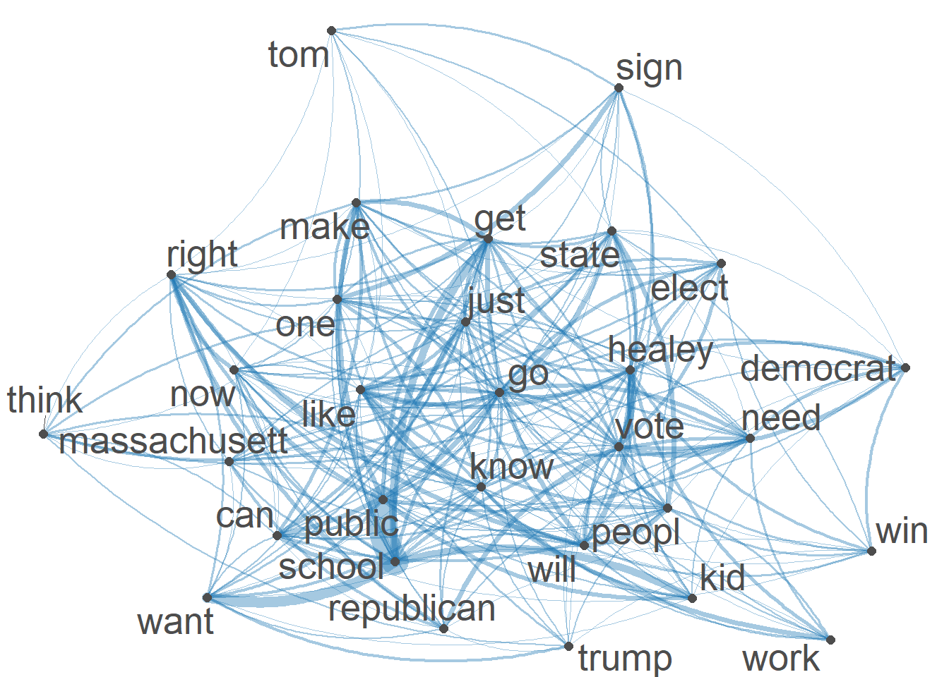

Code

fcm_select(Diehltopgat_fcm, pattern = Diehltoptag) %>%
    textplot_network(min_freq = 0.7, vertex_labelcolor = rep(c('black', NA), 15),vertex_labelsize = 6)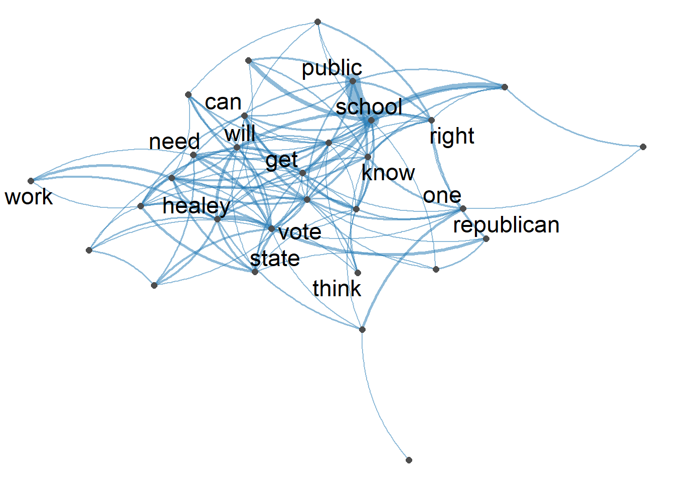

Code

D_csv <- as.data.frame((cbind(Diehl,Diehl_text_df)))
write_csv(D_csv,"D_csv")

Sentiment Analysis

NRC Dictionary

Code

#convert cleaned Diehl_tokens back tp corpus for sentiment analysis
Diehl_corpus <- corpus(as.character(Diehl_tokens))

# use liwcalike() to estimate sentiment using NRC dictionary
DiehlTweetSentiment_nrc <- liwcalike(Diehl_corpus, data_dictionary_NRC)

names(DiehlTweetSentiment_nrc)

 [1] "docname"      "Segment"      "WPS"          "WC"           "Sixltr"      
 [6] "Dic"          "anger"        "anticipation" "disgust"      "fear"        
[11] "joy"          "negative"     "positive"     "sadness"      "surprise"    
[16] "trust"        "AllPunc"      "Period"       "Comma"        "Colon"       
[21] "SemiC"        "QMark"        "Exclam"       "Dash"         "Quote"       
[26] "Apostro"      "Parenth"      "OtherP"

Code

DiehlTweetSentiment_nrc_viz <- DiehlTweetSentiment_nrc %>%
  select(c("anger", "anticipation", "disgust", "fear","joy","sadness", "surprise","trust","positive","negative"))


Diehl_tr<-data.frame(t(DiehlTweetSentiment_nrc_viz)) #transpose

Diehl_tr_new <- data.frame(rowSums(Diehl_tr[2:497]))
Diehl_tr_mean <- data.frame(rowMeans(Diehl_tr[2:497]))#get mean of sentiment values
names(Diehl_tr_new)[1] <- "Count"
Diehl_tr_new <- cbind("sentiment" = rownames(Diehl_tr_new), Diehl_tr_new)
rownames(Diehl_tr_new) <- NULL
Diehl_tr_new2<-Diehl_tr_new[1:8,]
write_csv(Diehl_tr_new2,"Diehl- 8 Sentiments")

Code

#Plot One - Count of words associated with each sentiment
quickplot(sentiment, data=Diehl_tr_new2, weight=Count, geom="bar", fill=sentiment, ylab="count")+ggtitle("Emotions to REPLIES Geoff Diehl Tweets")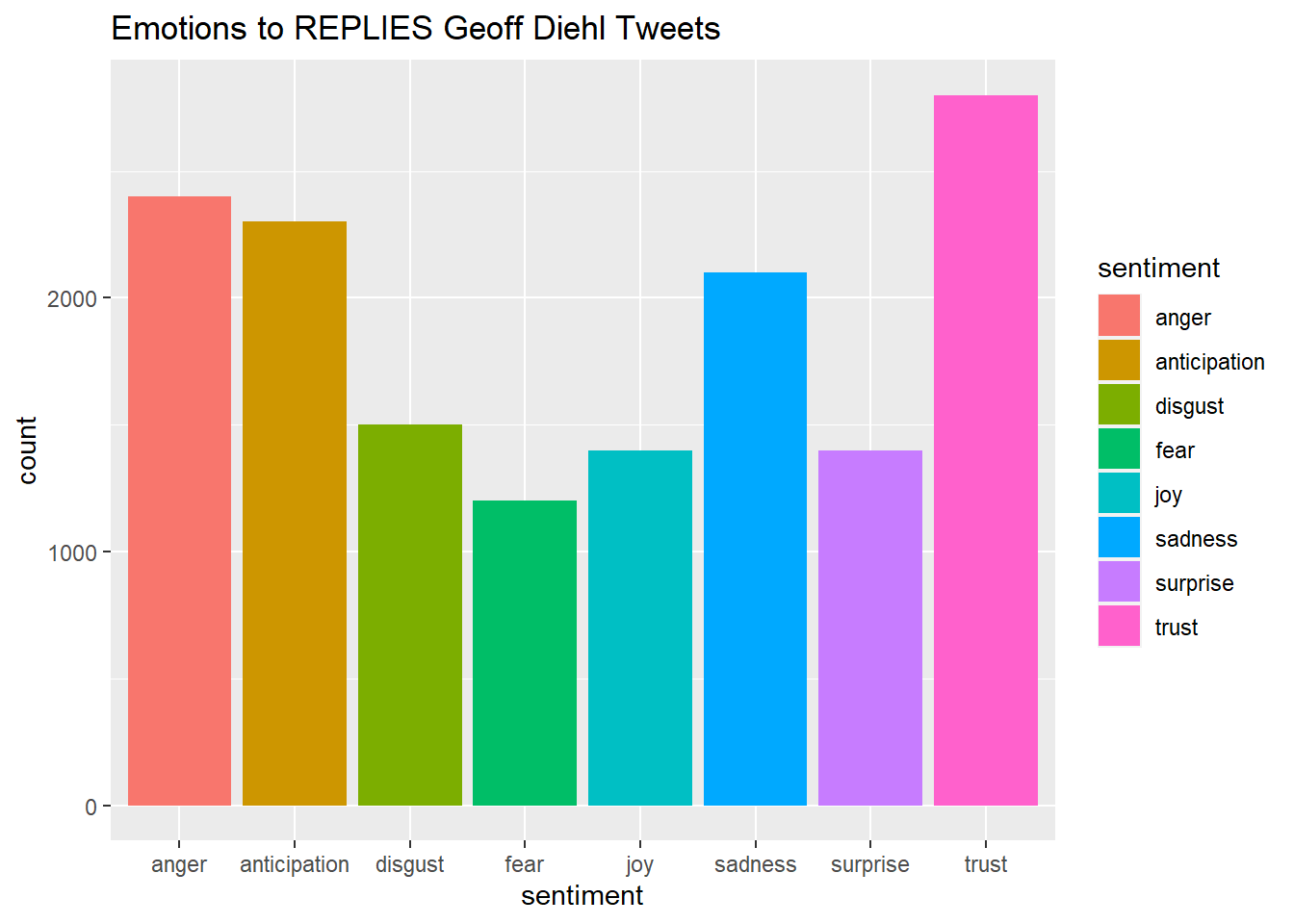

Code

names(Diehl_tr_mean)[1] <- "Mean"
Diehl_tr_mean <- cbind("sentiment" = rownames(Diehl_tr_mean), Diehl_tr_mean)
rownames(Diehl_tr_mean) <- NULL
Diehl_tr_mean2<-Diehl_tr_mean[9:10,]
write_csv(Diehl_tr_mean2,"Diehl -Mean Sentiments")

Code

#Plot One - Count of words associated with each sentiment
quickplot(sentiment, data=Diehl_tr_mean2, weight=Mean, geom="bar", fill=sentiment, ylab="Mean Sentiment Score")+ggtitle("Mean Sentiment Scores to Geoff Diehl Tweets")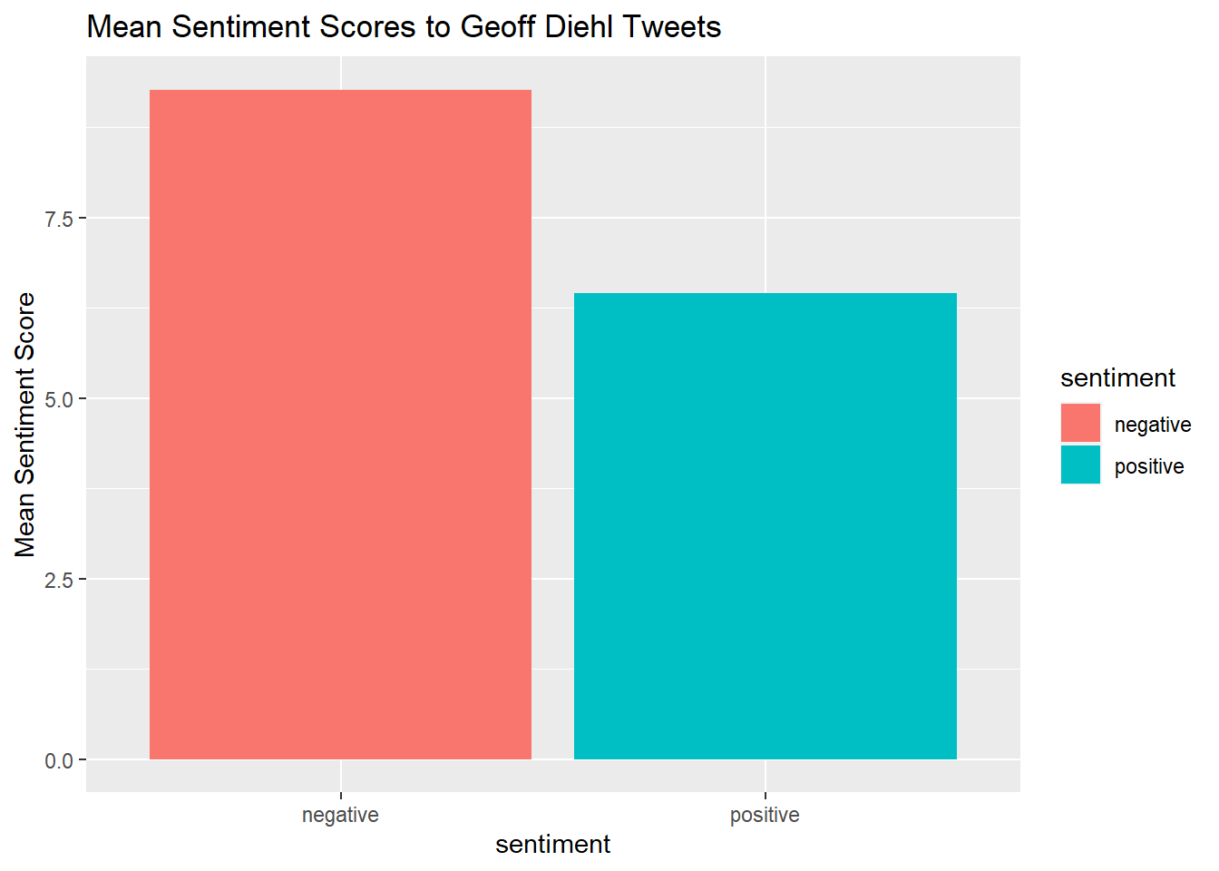

Polarity Scores

Code

Diehldf_nrc <- convert(DiehlDfm_nrc, to = "data.frame")
write_csv(Diehldf_nrc, "Diehl- Polarity Scores")

Diehldf_nrc$polarity <- (Diehldf_nrc$positive - Diehldf_nrc$negative)/(Diehldf_nrc$positive + Diehldf_nrc$negative)

Diehldf_nrc$polarity[(Diehldf_nrc$positive + Diehldf_nrc$negative) == 0] <- 0

ggplot(Diehldf_nrc) +
  geom_histogram(aes(x=polarity)) +
  theme_bw()

`stat_bin()` using `bins = 30`. Pick better value with `binwidth`.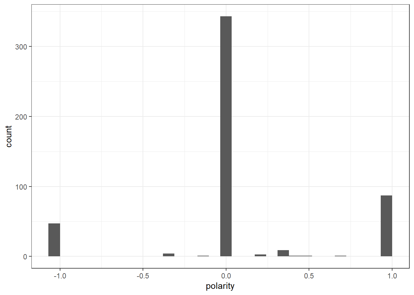

Bind to new DF

Code

Diehl_text_df <-as.data.frame(Diehl_text_df)
DiehlCorpus_Polarity <-as.data.frame((cbind(Diehldf_nrc,Diehl_text_df)))

subset to polarity and text

Code

DiehlCorpus_Polarity <- DiehlCorpus_Polarity %>%
  select(c("polarity","Diehl_corpus"))


DiehlCorpus_Polarity$polarity <- recode(DiehlCorpus_Polarity$polarity,
                                        "1" = "positive",
                                        "-1" = "negative",
                                        "0" = "neutral",)

Cleaned DF

Code

DiehlCorpus_Polarity <- na.omit(DiehlCorpus_Polarity)
head(DiehlCorpus_Polarity)

      polarity
text1  neutral
text2 negative
text3  neutral
text4 positive
text5 negative
text6 positive
                                                                                                                                                                                                                  Diehl_corpus
text1                                                                                                                                                                                           still beats fascism day week 📴
text2                                                                                                                                                                                                       wear mask ’re dumb
text3                                                                                     ’ mentioning masks paying companies can charge whatever want follow ’ll see shareholders companies keep voting party like dumb poor…
text4  argument gas pipelines energy independence right now new england gets lng deliveries international shipments nthese corporations making profit another story vg blckrck use public funds turn profit pull public money 
text5                                                                                                         shit u dumb masker democrats still fucked everyone caused price hikes higher taxes fn maskers u don’t know squat
text6                                                                     companies take profit loss kinder morgan elected need proof energy independence way actually take control prices give billionaires httpstcodairdldph

New Corpus with polarity scores

Code

DiehlCorpus_P<- corpus(DiehlCorpus_Polarity,text_field = "Diehl_corpus")

Sentiment Analysis

Polarity Scores

Code

Diehldf_nrc <- convert(DiehlDfm_nrc, to = "data.frame")
write_csv(Diehldf_nrc, "Diehl- Polarity Scores")

Diehldf_nrc$polarity <- (Diehldf_nrc$positive - Diehldf_nrc$negative)/(Diehldf_nrc$positive + Diehldf_nrc$negative)

Diehldf_nrc$polarity[(Diehldf_nrc$positive + Diehldf_nrc$negative) == 0] <- 0

ggplot(Diehldf_nrc) +
  geom_histogram(aes(x=polarity)) +
  theme_bw()

`stat_bin()` using `bins = 30`. Pick better value with `binwidth`.

Bind to new DF

Code

Diehl_text_df <-as.data.frame(Diehl_text_df)
DiehlCorpus_Polarity <-as.data.frame((cbind(Diehldf_nrc,Diehl_text_df)))

subset to polarity and text

Code

DiehlCorpus_Polarity <- DiehlCorpus_Polarity %>%
  select(c("polarity","Diehl_corpus"))


DiehlCorpus_Polarity$polarity <- recode(DiehlCorpus_Polarity$polarity,
                                        "1" = "positive",
                                        "-1" = "negative",
                                        "0" = "neutral",)

FOCUS: SENTIMENT ANALYSIS

HEALEY DATA

Code

library(ggplot2)
library(lubridate)
library(reshape2)


Attaching package: 'reshape2'

The following object is masked from 'package:tidyr':

    smiths

Code

library(dplyr)
library(syuzhet) 
library(stringr)
library(tidyr)
library(DT)

Code

Healy_csv <- read.csv("H_csv")

datatable(Healy_csv[1:50,], options = list(pageLength = 5))

Code

Healy_csv$created_at <- ymd_hms(Healy_csv$created_at) 
Healy_csv$created_at <- with_tz(Healy_csv$created_at,"America/New_York")
Healy_csv$created_date <- as.Date(Healy_csv$created_at)

Code

HealySentiment <- get_nrc_sentiment(Healy_csv$text) 
Hall_senti <- cbind(Healy_csv, HealySentiment)  #Combine sentiment ratings to create a new data frame

#show 50 messages rated by the NRC dictionary. 
datatable(Hall_senti[1:50,17:29], options = list(pageLength = 5))

Code

### Summary statistics by group variables
Hall_senti$date_label <- as.factor(Hall_senti$created_date)

Hsenti_aggregated <- Hall_senti %>% 
  dplyr::group_by(date_label) %>%
  dplyr::summarise(anger = mean(anger), 
            anticipation = mean(anticipation), 
            disgust = mean(disgust), 
            fear = mean(fear), 
            joy = mean(joy), 
            sadness = mean(sadness), 
            surprise = mean(surprise), 
            trust = mean(trust)) 

Hsenti_aggregated <- Hsenti_aggregated %>% pivot_longer(cols = -c(date_label), names_to = "variable", values_to = "value")

datatable(Hsenti_aggregated[1:50,], options = list(pageLength = 5))

Code

Hsenti_aggregated$date_label <- as.Date(Hsenti_aggregated$date_label)

ggplot(data = Hsenti_aggregated, aes(x = date_label, y = value)) +
  geom_line(size = 2, alpha = 2, aes(color = variable)) +
  geom_point(size = 0) +
  ylim(0, NA) +
  theme(legend.title=element_blank(), axis.title.x = element_blank()) +
  ylab("Average sentiment score") + 
  ggtitle("Sentiments on HEALEY Tweets before Election Day")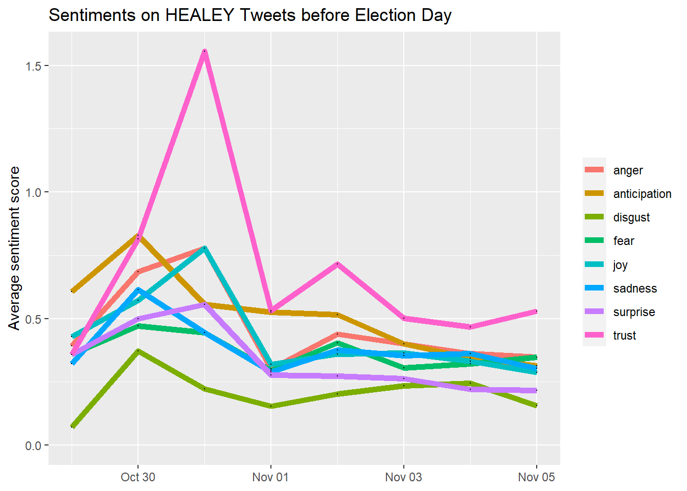

Code

library(highcharter)

Registered S3 method overwritten by 'quantmod':
  method            from
  as.zoo.data.frame zoo

Code

title <- paste0("sentiment scores over time", Sys.Date())
highchart() %>%
  hc_add_series(Hsenti_aggregated,"line", hcaes(x = date_label, y = value,group=variable)) %>%
  hc_xAxis(type = "datetime") %>%
   hc_title(
    text = "Sentiments on Healey Tweets Before Election Day",
    margin = 10,
    align = "center",
    style = list(color = "Black", useHTML = TRUE)
  )

Code

library(tidytext)
library(textdata)

Error in library(textdata): there is no package called 'textdata'

Code

library(tidyr)

Hcsv_clean <- Healy_csv %>%
  dplyr::select(text) %>%
  unnest_tokens(word, text)

Hsentiment_word_counts <- Hcsv_clean %>%
  inner_join(get_sentiments("nrc")) %>%
  dplyr::count(word, sentiment, sort = TRUE) %>%
  ungroup()

Error: The textdata package is required to download the NRC word-emotion association lexicon.
Install the textdata package to access this dataset.

visualize key sentimental terms

Code

Hsentiment_word_counts %>%
  group_by(sentiment) %>%
  top_n(5) %>%
  ungroup() %>%
  mutate(word = reorder(word, n)) %>%
  ggplot(aes(word, n, fill = sentiment)) +
  geom_col(show.legend = FALSE) +
  facet_wrap(~sentiment, scales = "free_y") +
  labs(title = "Healey Tweet Replies Contribution to Sentiment",
       y = "Contribution to sentiment",
       x = NULL) +
  coord_flip()

Error in group_by(., sentiment): object 'Hsentiment_word_counts' not found

DIEHL DATA

Code

Diehl_csv <- read.csv("D_csv")

datatable(Diehl_csv[1:50,], options = list(pageLength = 5))

Code

Diehl_csv$created_at <- ymd_hms(Diehl_csv$created_at) 
Diehl_csv$created_at <- with_tz(Diehl_csv$created_at,"America/New_York")
Diehl_csv$created_date <- as.Date(Diehl_csv$created_at)

Code

DiehlSentiment <- get_nrc_sentiment(Diehl_csv$text) 
Dall_senti <- cbind(Diehl_csv, DiehlSentiment)  #Combine sentiment ratings to create a new data frame

#show 50 messages rated by the NRC dictionary. 
datatable(Dall_senti[1:50,17:29], options = list(pageLength = 5))

Code

### Summary statistics by group variables
Dall_senti$date_label <- as.factor(Dall_senti$created_date)

Dsenti_aggregated <- Dall_senti %>% 
  dplyr::group_by(date_label) %>%
  dplyr::summarise(anger = mean(anger), 
            anticipation = mean(anticipation), 
            disgust = mean(disgust), 
            fear = mean(fear), 
            joy = mean(joy), 
            sadness = mean(sadness), 
            surprise = mean(surprise), 
            trust = mean(trust)) 

Dsenti_aggregated <- Dsenti_aggregated %>% pivot_longer(cols = -c(date_label), names_to = "variable", values_to = "value")

datatable(Dsenti_aggregated[1:50,], options = list(pageLength = 5))

Code

Dsenti_aggregated$date_label <- as.Date(Dsenti_aggregated$date_label)

ggplot(data = Dsenti_aggregated, aes(x = date_label, y = value)) +
  geom_line(size = 2, alpha = 2, aes(color = variable)) +
  geom_point(size = 0) +
  ylim(0, NA) +
  theme(legend.title=element_blank(), axis.title.x = element_blank()) +
  ylab("Average sentiment score") + 
  ggtitle("Sentiments on DIEHL Tweets before Election Day")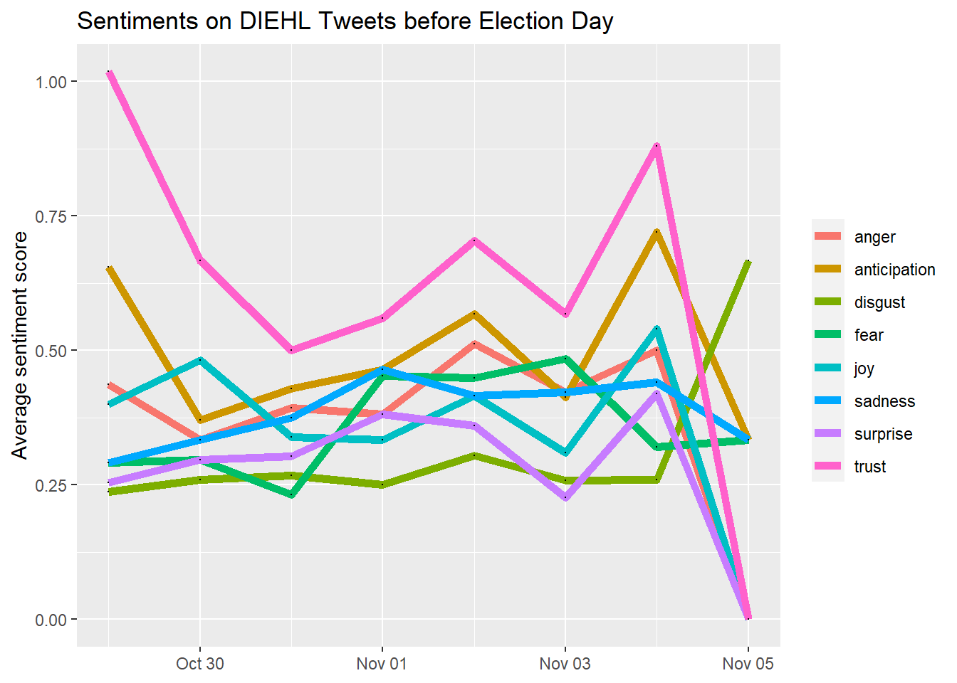

Code

library(highcharter)
title <- paste0("sentiment scores over time", Sys.Date())
highchart() %>%
  hc_add_series(Dsenti_aggregated,"line", hcaes(x = date_label, y = value,group=variable)) %>%
  hc_xAxis(type = "datetime") %>%
   hc_title(
    text = "Sentiments on DIEHL Tweets Before Election Day",
    margin = 10,
    align = "center",
    style = list(color = "Black", useHTML = TRUE)
  )

Code

library(tidytext)
library(textdata)

Error in library(textdata): there is no package called 'textdata'

Code

library(tidyr)

Dcsv_clean <- Diehl_csv %>%
  dplyr::select(text) %>%
  unnest_tokens(word, text)

Dsentiment_word_counts <- Dcsv_clean %>%
  inner_join(get_sentiments("nrc")) %>%
  dplyr::count(word, sentiment, sort = TRUE) %>%
  ungroup()

Error: The textdata package is required to download the NRC word-emotion association lexicon.
Install the textdata package to access this dataset.

visualize key sentimental terms

Code

Dsentiment_word_counts %>%
  group_by(sentiment) %>%
  top_n(5) %>%
  ungroup() %>%
  mutate(word = reorder(word, n)) %>%
  ggplot(aes(word, n, fill = sentiment)) +
  geom_col(show.legend = FALSE) +
  facet_wrap(~sentiment, scales = "free_y") +
  labs(title = "DIEHL Tweet Replies Contribution to Sentiment",
       y = "Words Contribution to Sentiments",
       x = NULL) +
  coord_flip()

Error in group_by(., sentiment): object 'Dsentiment_word_counts' not found