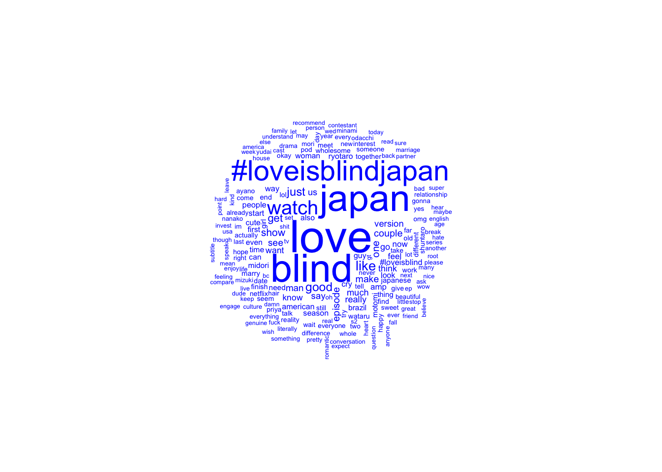
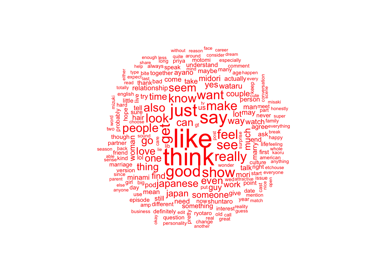
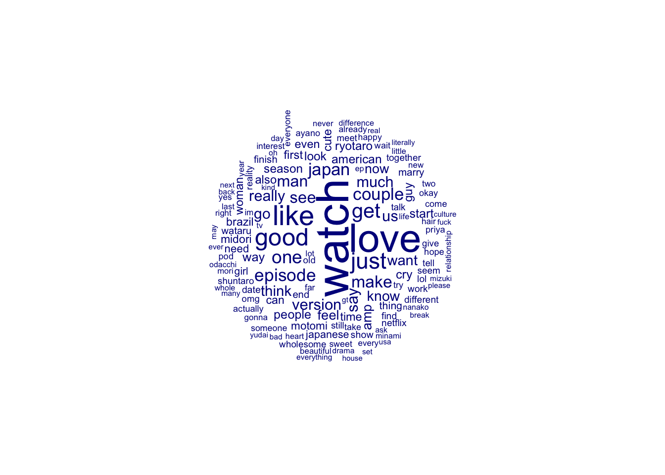
Although the data is a lot cleaner now I do wonder if removing the key words “love”, “blind”, “japan” and “#loveisblindjapan” will give a better picture of how posters are feeling. I will go ahead and remove the phrases.
Here is we can see a more accurate idea of how people are tweeting about the show. Even with the show’s title being remove love is still a large part of tweets.
I also noticed that “blind” was used often. Looking at the tweets it seems unlikely that the word blind was used in any other way than to mention the show. Thus I’d like to remove the word blind as well since it seems unlikely to be useful to sentiment analysis.
I will also remove the word “show” as show seemingly is only talking about the series rather than any emotions.
I have also found a different way to remove dates and have done so below.
I have found out why the dates column has become messy. This is because originally I had put the corpus() function after the [!is.na()]. However when put first it still shows the date column in the summary.
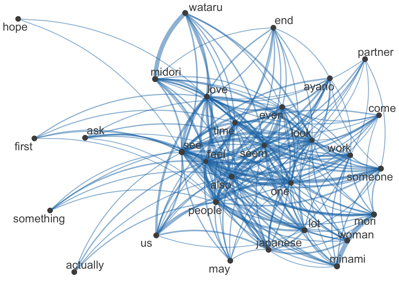
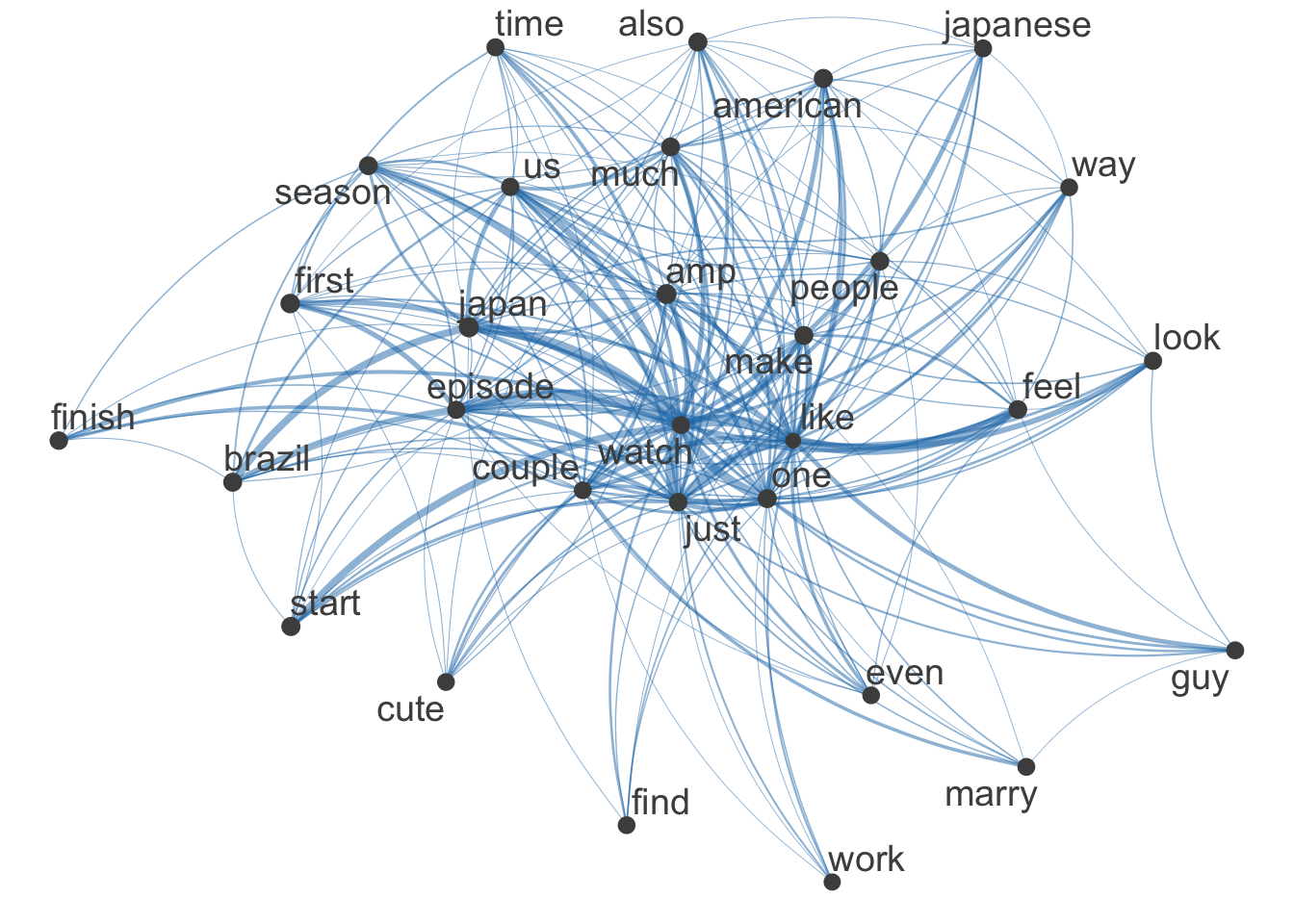
I mentioned previously I would like to test a textplot for Reddit. Below you will see my test.
Code
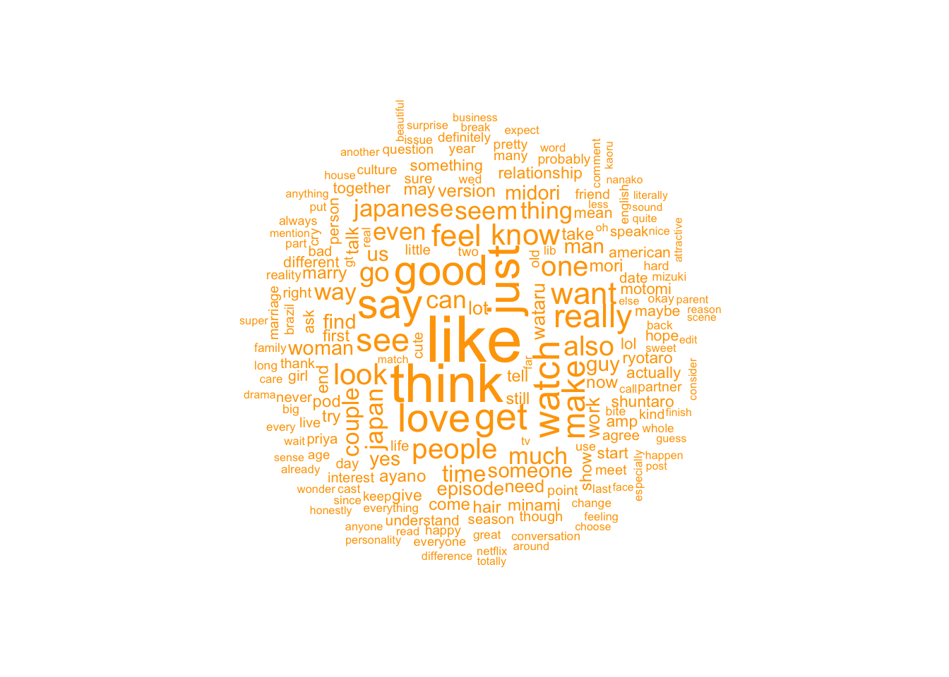
# let's create a nicer dfm by limiting to words that appear frequently and are in more than 30% of chaptersrsmaller_dfm <-dfm_trim(reddit_corpus_dfm, max_termfreq =3400, min_termfreq =10)rsmaller_dfm <-dfm_trim(rsmaller_dfm, max_docfreq = .3, docfreq_type ="prop")textplot_wordcloud(rsmaller_dfm, min_count =100,random_order =FALSE)
Code
# create fcm from dfmrsmaller_fcm <-fcm(rsmaller_dfm)# check the dimensions (i.e., the number of rows and the number of columnns)# of the matrix we createddim(rsmaller_fcm)
[1] 1185 1185
Code
rmyFeatures <-names(topfeatures(rsmaller_fcm, 30))# retain only those top features as part of our matrixreven_smaller_fcm <-fcm_select(rsmaller_fcm, pattern = rmyFeatures, selection ="keep")# check dimensionsdim(reven_smaller_fcm)
[1] 30 30
Code
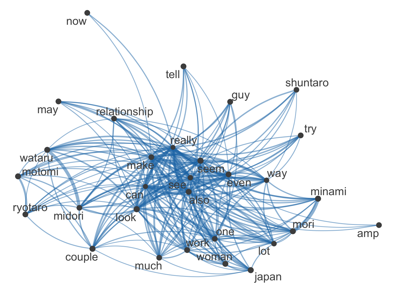
# compute size weight for vertices in networkrsize <-log(colSums(reven_smaller_fcm))# create plottextplot_network(reven_smaller_fcm, vertex_size = rsize /max(rsize) *3)
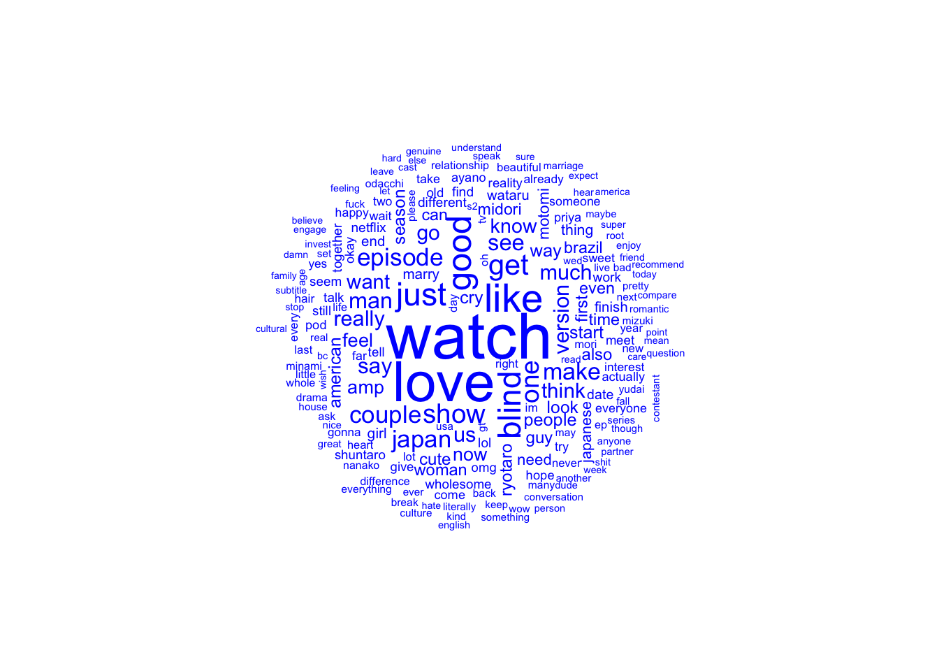
It’s interesting to see that the contestants names seem to be much more connected. Overall Reddit’s text plot feels a lot more interconnected than Twitter’s.
I will also test this for the combined data set.
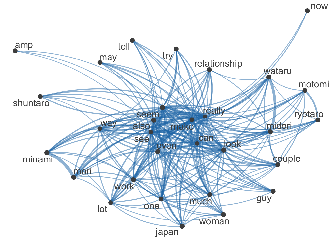
All Social Media Tex Plot
Code
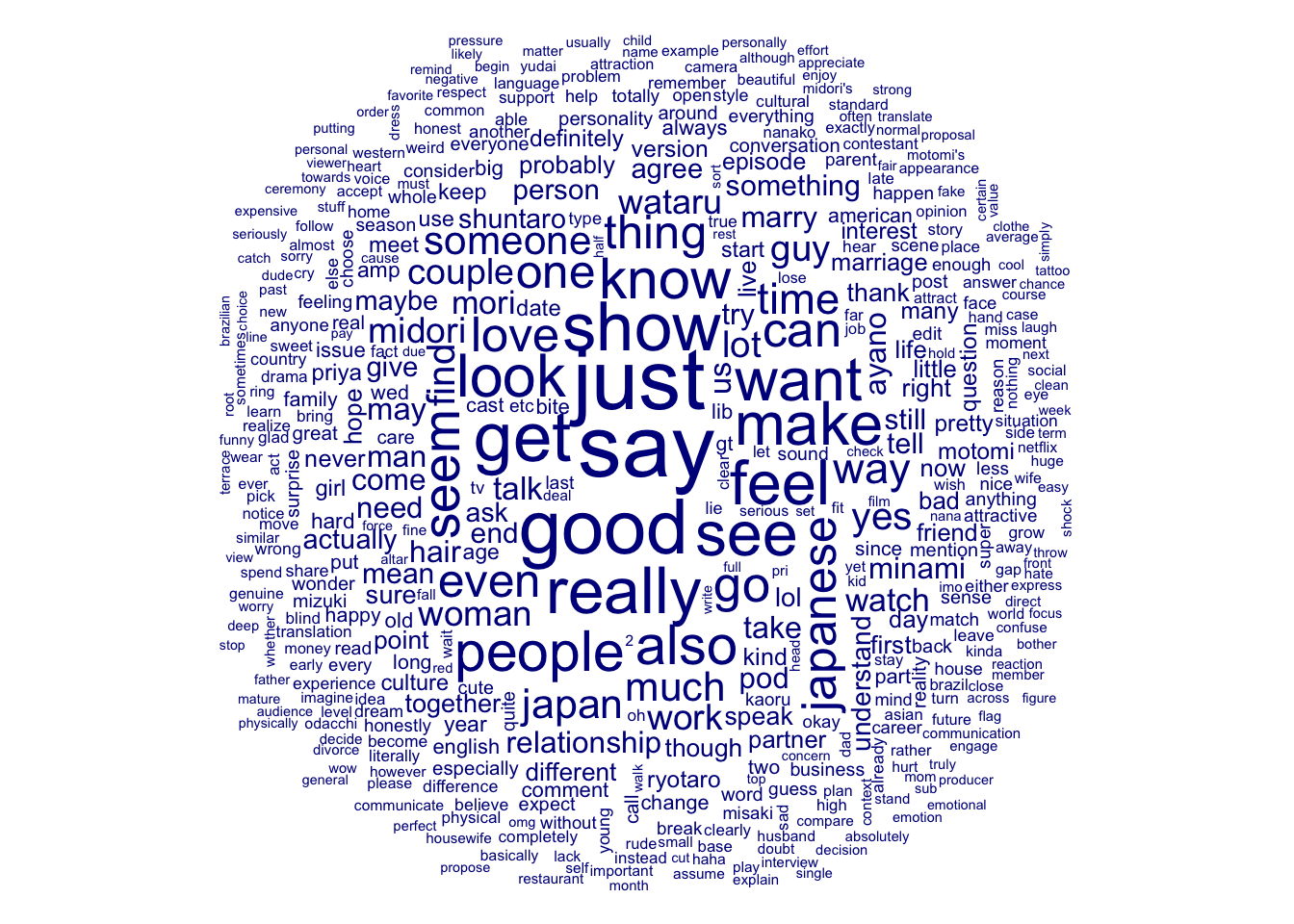
# let's create a nicer dfm by limiting to words that appear frequently and are in more than 30% of chaptersssmaller_dfm <-dfm_trim(social_corpus_dfm, max_termfreq =3400, min_termfreq =10)ssmaller_dfm <-dfm_trim(ssmaller_dfm, max_docfreq = .3, docfreq_type ="prop")textplot_wordcloud(ssmaller_dfm, min_count =100,random_order =FALSE)
Code
# create fcm from dfmssmaller_fcm <-fcm(ssmaller_dfm)# check the dimensions (i.e., the number of rows and the number of columnns)# of the matrix we createddim(ssmaller_fcm)
[1] 1405 1405
Code
smyFeatures <-names(topfeatures(ssmaller_fcm, 30))# retain only those top features as part of our matrixseven_smaller_fcm <-fcm_select(ssmaller_fcm, pattern = smyFeatures, selection ="keep")# check dimensionsdim(seven_smaller_fcm)
[1] 30 30
Code
# compute size weight for vertices in networkssize <-log(colSums(seven_smaller_fcm))# create plottextplot_network(seven_smaller_fcm, vertex_size = ssize /max(ssize) *3)
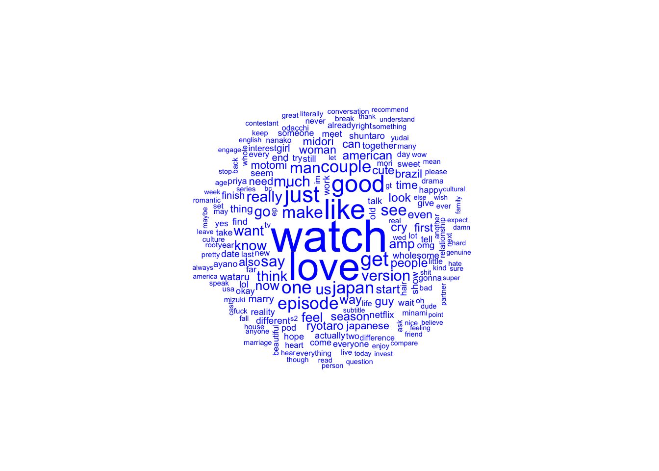
Interestingly the text plot has a similarity more to Reddit than to Twitter. Perhaps this is because Reddit has more tokens as there is not a character limit.
Dictionary Approach with Twitter
I will now try the dictionary approach using reddit, twitter, and the data combined (allsocialmedia).
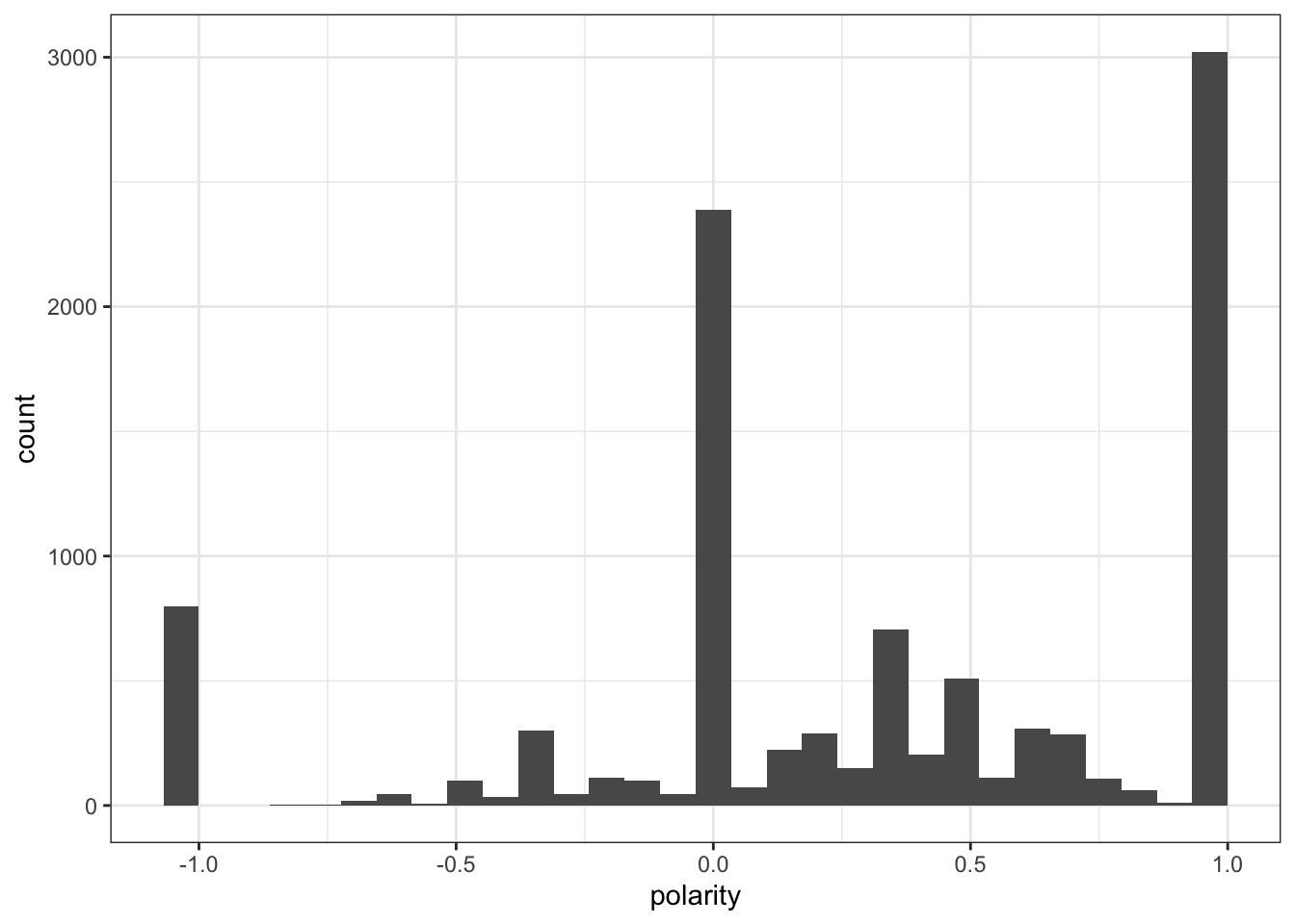
`stat_bin()` using `bins = 30`. Pick better value with `binwidth`.
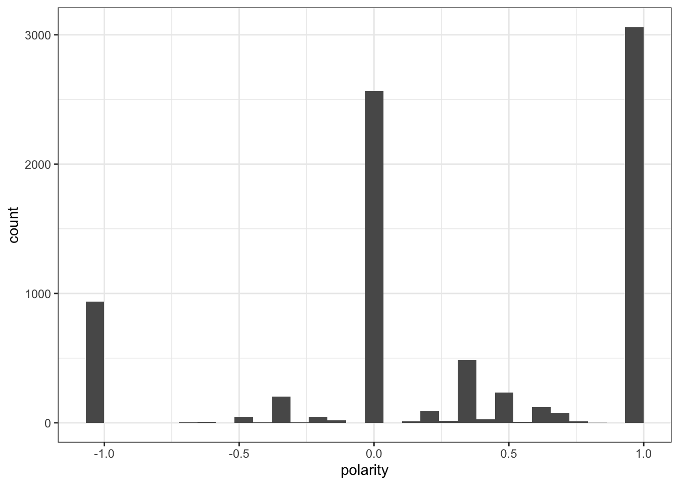
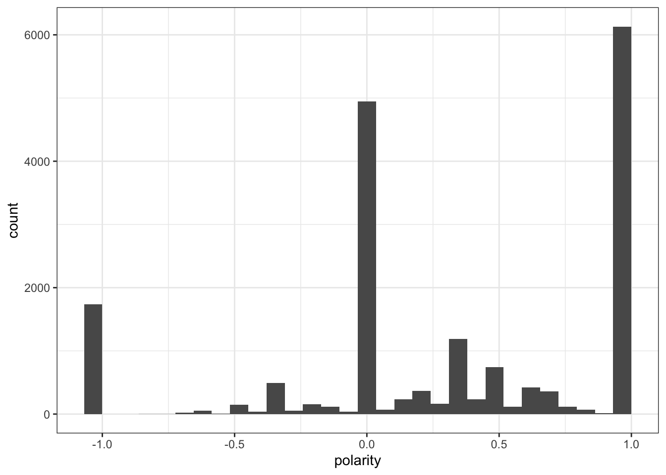
Here we can see that for twitter most people were more positive about the show! That does correlate from what I often saw from skimming the tweets.
Still we should double check to make sure that these actually do skew positively.
Code
# convert corpus to DFM using the LSD2015 dictionarytwitterDfm_lsd2015 <-dfm(tokens(twitter_text_lemmitized, remove_punct =TRUE),tolower =TRUE) %>%dfm_lookup(data_dictionary_LSD2015)# convert corpus to DFM using the General Inquirer dictionarytwitterDfm_geninq <-dfm(tokens(twitter_text_lemmitized, remove_punct =TRUE),tolower =TRUE) %>%dfm_lookup(data_dictionary_geninqposneg)# create polarity measure for LSD2015tdf_lsd2015 <-convert(twitterDfm_lsd2015, to ="data.frame")tdf_lsd2015$polarity <- (tdf_lsd2015$positive - tdf_lsd2015$negative)/(tdf_lsd2015$positive + tdf_lsd2015$negative)tdf_lsd2015$polarity[which((tdf_lsd2015$positive + tdf_lsd2015$negative) ==0)] <-0# look at first few rowshead(tdf_lsd2015)
# create polarity measure for GenInqtdf_geninq <-convert(twitterDfm_geninq, to ="data.frame")tdf_geninq$polarity <- (tdf_geninq$positive - tdf_geninq$negative)/(tdf_geninq$positive + tdf_geninq$negative)tdf_geninq$polarity[which((tdf_geninq$positive + tdf_geninq$negative) ==0)] <-0# look at first few rowshead(tdf_geninq)
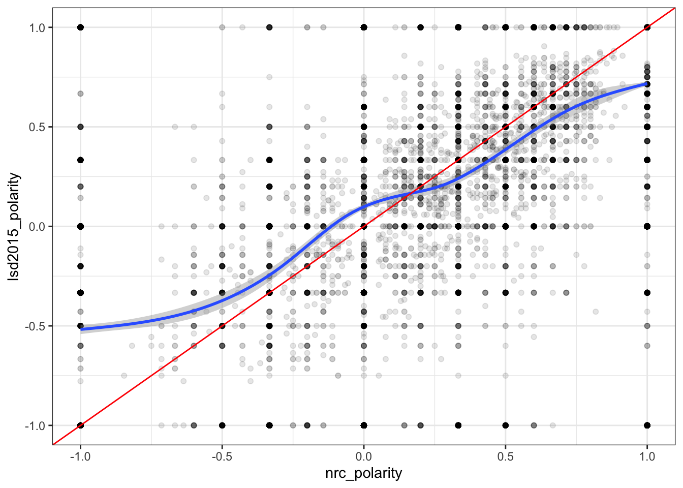
# Plot these out. You can update this to check the look of other combinationsggplot(tsent_df, mapping =aes(x=nrc_polarity, y=lsd2015_polarity)) +geom_point(alpha =0.1) +geom_smooth() +geom_abline(intercept=0,slope=1, color ="red") +theme_bw()
`geom_smooth()` using method = 'gam' and formula 'y ~ s(x, bs = "cs")'
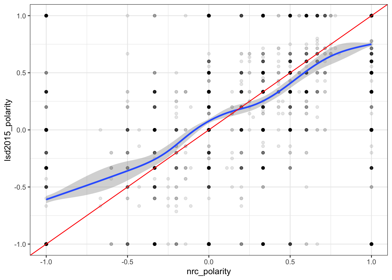
Interestingly it seems there is a good amount of correlation between the two. Although not as strong as the tutorial it does seem that the dictionary is fairly accurate. Let’s test this for both reddit and allsocialmedia.
`stat_bin()` using `bins = 30`. Pick better value with `binwidth`.
Code
# convert corpus to DFM using the LSD2015 dictionaryredditDfm_lsd2015 <-dfm(tokens(reddit_lemmitized, remove_punct =TRUE),tolower =TRUE) %>%dfm_lookup(data_dictionary_LSD2015)# convert corpus to DFM using the General Inquirer dictionaryredditDfm_geninq <-dfm(tokens(reddit_lemmitized, remove_punct =TRUE),tolower =TRUE) %>%dfm_lookup(data_dictionary_geninqposneg)# create polarity measure for LSD2015rdf_lsd2015 <-convert(redditDfm_lsd2015, to ="data.frame")rdf_lsd2015$polarity <- (rdf_lsd2015$positive - rdf_lsd2015$negative)/(rdf_lsd2015$positive + rdf_lsd2015$negative)rdf_lsd2015$polarity[which((rdf_lsd2015$positive + rdf_lsd2015$negative) ==0)] <-0# look at first few rowshead(rdf_lsd2015)
# create polarity measure for GenInqrdf_geninq <-convert(redditDfm_geninq, to ="data.frame")rdf_geninq$polarity <- (rdf_geninq$positive - rdf_geninq$negative)/(rdf_geninq$positive + rdf_geninq$negative)rdf_geninq$polarity[which((rdf_geninq$positive + rdf_geninq$negative) ==0)] <-0# look at first few rowshead(rdf_geninq)
# Plot these out. You can update this to check the look of other combinationsggplot(rsent_df, mapping =aes(x=nrc_polarity, y=lsd2015_polarity)) +geom_point(alpha =0.1) +geom_smooth() +geom_abline(intercept=0,slope=1, color ="red") +theme_bw()
`geom_smooth()` using method = 'gam' and formula 'y ~ s(x, bs = "cs")'
`stat_bin()` using `bins = 30`. Pick better value with `binwidth`.
Code
# convert corpus to DFM using the LSD2015 dictionarysocialDfm_lsd2015 <-dfm(tokens(social_lemmitized, remove_punct =TRUE),tolower =TRUE) %>%dfm_lookup(data_dictionary_LSD2015)# convert corpus to DFM using the General Inquirer dictionarysocialDfm_geninq <-dfm(tokens(social_lemmitized, remove_punct =TRUE),tolower =TRUE) %>%dfm_lookup(data_dictionary_geninqposneg)# create polarity measure for LSD2015df_lsd2015 <-convert(socialDfm_lsd2015, to ="data.frame")df_lsd2015$polarity <- (df_lsd2015$positive - df_lsd2015$negative)/(df_lsd2015$positive + df_lsd2015$negative)df_lsd2015$polarity[which((df_lsd2015$positive + df_lsd2015$negative) ==0)] <-0# look at first few rowshead(df_lsd2015)
# create polarity measure for GenInqdf_geninq <-convert(socialDfm_geninq, to ="data.frame")df_geninq$polarity <- (df_geninq$positive - df_geninq$negative)/(df_geninq$positive + df_geninq$negative)df_geninq$polarity[which((df_geninq$positive + df_geninq$negative) ==0)] <-0# look at first few rowshead(df_geninq)
# Plot these out. You can update this to check the look of other combinationsggplot(sent_df, mapping =aes(x=nrc_polarity, y=lsd2015_polarity)) +geom_point(alpha =0.1) +geom_smooth() +geom_abline(intercept=0,slope=1, color ="red") +theme_bw()
`geom_smooth()` using method = 'gam' and formula 'y ~ s(x, bs = "cs")'
Choosing a Dictionary
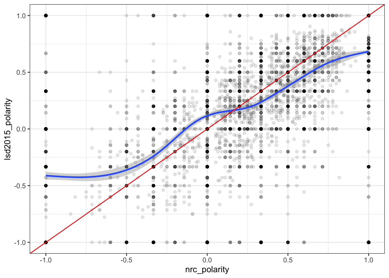
Interestingly compared to Twitter, Reddit and “allsocialmedia” were a fair amount lower in correlation. Although it was still a fairly high correlation this may because of the different types of words used by Reddit.
However when you compare the graphs all three are nearly identical in nature.
I think I will use the NRC dictionary. I have chosen this one because I believe it’s the strongest dictionary for my set of data because it explores through multiple categories of emotions. While both other dictionaries are good, NRC is a much larger dictionary. If you are interested I have found some more information on the dictionaries here!
Choosing a Research Question
After looking through all of the data using the dictionary method I have decided to go back to this research question: How do Reddit and Twitter users sentiment differentiate about the show Love is Blind Japan?
I have decided to do this because I believe there’s more information that could be compared. Additionally while it is useful to know an overall sentiment for social media, I think that since each user base may be different we could see more interesting results when it is not mixed together.
Final Thoughts (TLDR)
Final thoughts
I have found a way to keep the date column in the summary but remove it from the actual tokens afterwards.
I have made a list of stop words that are related to the title of the show from Twitter.
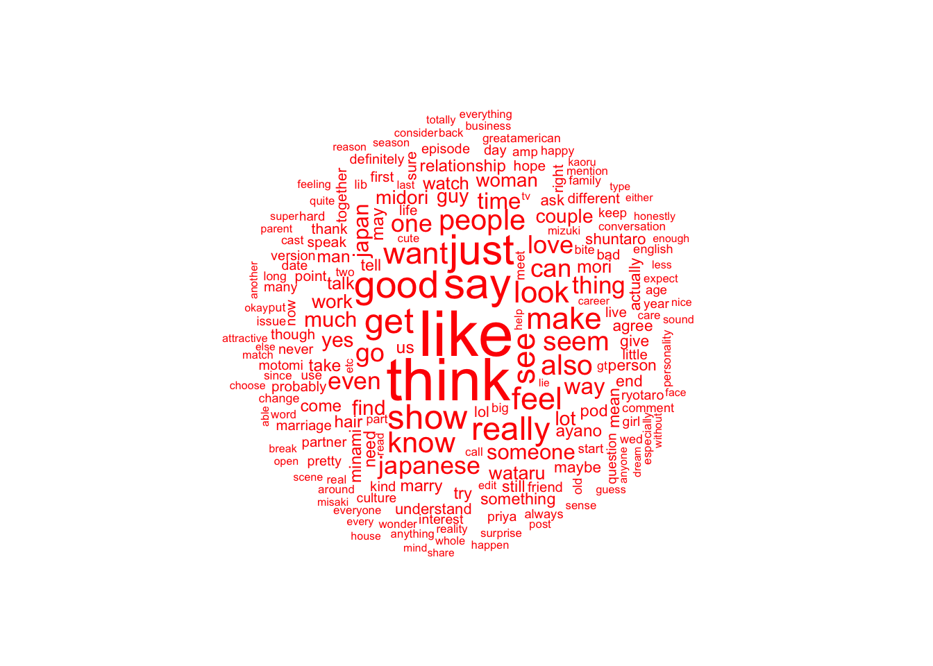
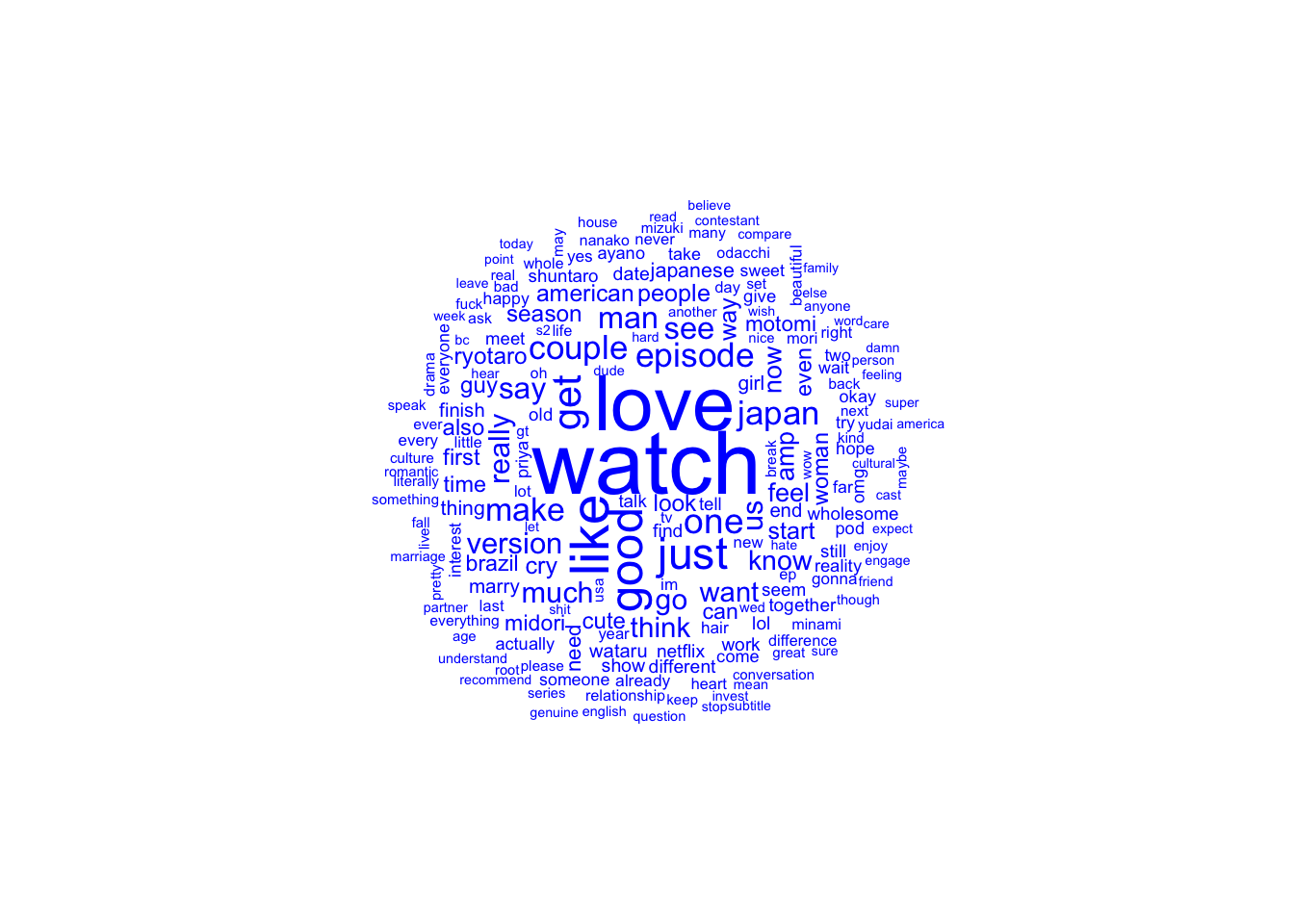
I have also included the removal of the word “show” as for tweets it only referenced show as a TV series. However for Reddit I have not removed the word show as Redditors seemed to use the word show outside of of meaning a TV show.
Reddit also did not have the same issues with the title of the show due to all of the posts in the sub reddit being related to Love is Blind Japan.
I have decided to use the NRC dictionary.
I have changed my question: How do Reddit and Twitter users sentiment differentiate about the show Love is Blind Japan?
This means I will no longer use the combined data set.
I am unsure how I will use co-occurrence.
Future Work
Here are a few things I’d like to do in blog post 5:
I would like to look at co-occurrence more closely and decide if the code I have now is the one I would like to use for the final project. I currently have chosen it based off prior issues (such as having the show’s name showing up).
This may include using a maxium document frequency and a minimum word frequency.
I would like to see if I can create an emotional rating comparison using the dictionary method. This would include using the NRC for twitter and reddit to compare the average emotional response.
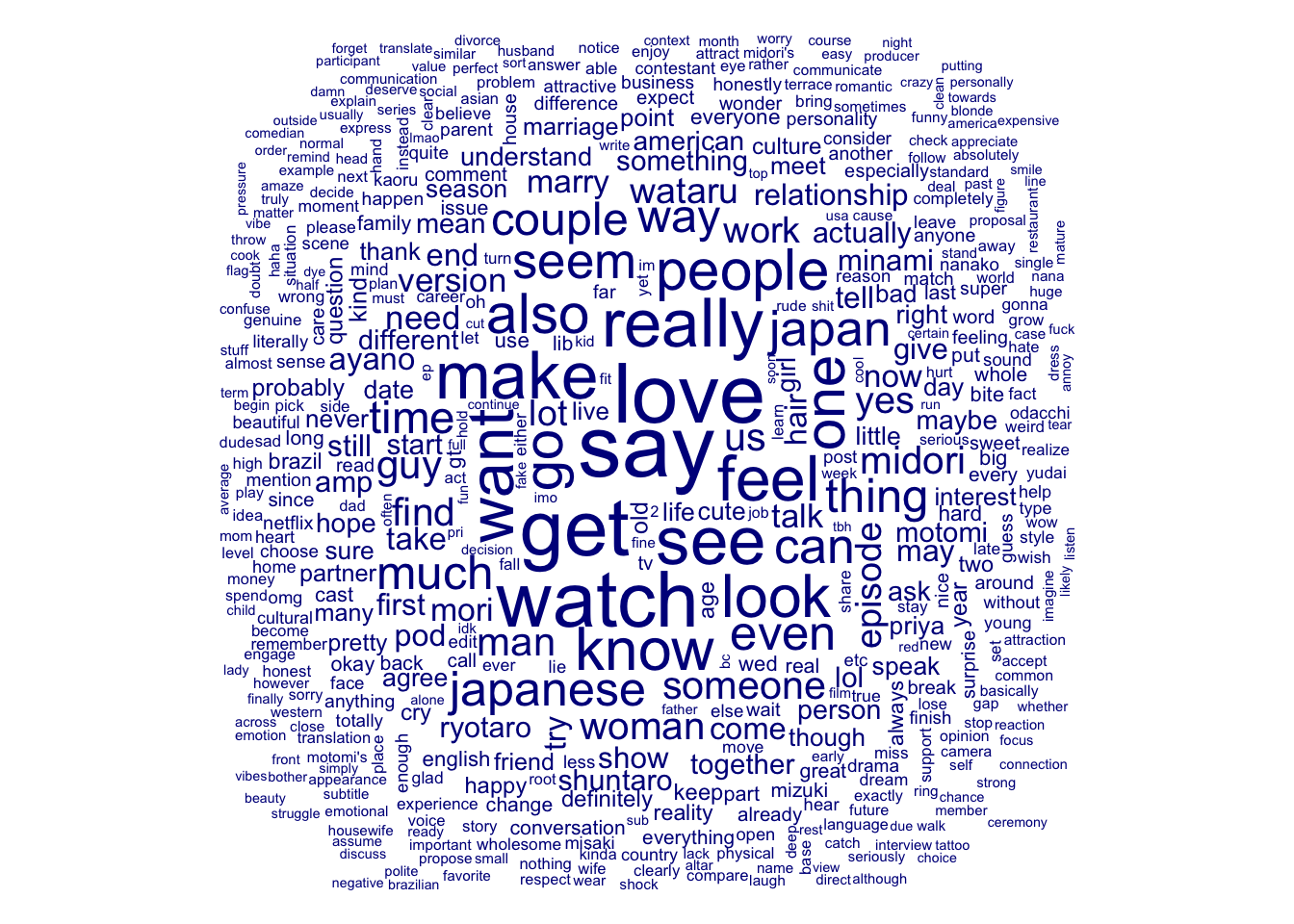
# let's create a nicer dfm by limiting to words that appear frequently and are in more than 30% of chapterssmaller_dfm <-dfm_trim(twitter_corpus_text_dfm, max_termfreq =3400, min_termfreq =10)smaller_dfm <-dfm_trim(smaller_dfm, max_docfreq = .3, docfreq_type ="prop")textplot_wordcloud(smaller_dfm, min_count =100,random_order =FALSE)
Code
# create fcm from dfmsmaller_fcm <-fcm(smaller_dfm)# check the dimensions (i.e., the number of rows and the number of columnns)# of the matrix we createddim(smaller_fcm)
[1] 440 440
Code
myFeatures <-names(topfeatures(smaller_fcm, 30))# retain only those top features as part of our matrixeven_smaller_fcm <-fcm_select(smaller_fcm, pattern = myFeatures, selection ="keep")# check dimensionsdim(even_smaller_fcm)
[1] 30 30
Code
# compute size weight for vertices in networksize <-log(colSums(even_smaller_fcm))# create plottextplot_network(even_smaller_fcm, vertex_size = size /max(size) *3)
Code
# let's create a nicer dfm by limiting to words that appear frequently and are in more than 30% of chaptersrsmaller_dfm <-dfm_trim(reddit_corpus_dfm, max_termfreq =3400, min_termfreq =10)rsmaller_dfm <-dfm_trim(rsmaller_dfm, max_docfreq = .3, docfreq_type ="prop")textplot_wordcloud(rsmaller_dfm, min_count =100,random_order =FALSE)
Code
# create fcm from dfmrsmaller_fcm <-fcm(rsmaller_dfm)# check the dimensions (i.e., the number of rows and the number of columnns)# of the matrix we createddim(rsmaller_fcm)
[1] 1185 1185
Code
rmyFeatures <-names(topfeatures(rsmaller_fcm, 30))# retain only those top features as part of our matrixreven_smaller_fcm <-fcm_select(rsmaller_fcm, pattern = rmyFeatures, selection ="keep")# check dimensionsdim(reven_smaller_fcm)
[1] 30 30
Code
# compute size weight for vertices in networkrsize <-log(colSums(reven_smaller_fcm))# create plottextplot_network(reven_smaller_fcm, vertex_size = rsize /max(rsize) *3)
`stat_bin()` using `bins = 30`. Pick better value with `binwidth`.
Source Code
---title: "Blog Post Four"author: "Molly Hackbarth"description: "Working with the data"date: "10/29/2022"format: html: toc: true code-fold: true code-copy: true code-tools: truecategories: - blog posts - hw4 - Molly Hackbarth---```{r}#| label: setup#| warning: falselibrary(tidyverse)library(cld3)library(dplyr)library(here)library(devtools)library(tidytext)library(quanteda)library(quanteda.textstats)library(quanteda.textmodels)library(quanteda.textplots)#new packages#devtools::install_github("kbenoit/quanteda.dictionaries") library(quanteda.dictionaries)#devtools::install_github("quanteda/quanteda.sentiment")library(quanteda.sentiment)knitr::opts_chunk$set(echo =TRUE)```# Research Question**My current research question:** How do Reddit and Twitter users feel about the show *Love is Blind Japan*?# Reading in the Data```{r reading data}#write csv has been commented out due to it continously trying to save an "updated version" in Git. reddit_data <-read.csv(here::here("posts", "_data", "loveisblindjapan.csv"))twitter1 <-read.csv(here::here("posts", "_data", "tweets.csv"))twitter2 <-read.csv(here::here("posts", "_data", "tweets#.csv"))reddit <-subset(reddit_data, select =c("body", "created_utc")) reddit$created_utc <-as.Date.POSIXct(reddit$created_utc)reddit <- reddit %>%select(text = body, date = created_utc)# remove deleted or removed comments by moderators of the subreddit (ones that only contain [deleted] or [removed])reddit <- reddit %>%filter(!text =='[deleted]') %>%filter(!text =='[removed]')#remove counting columntwitter1 <- twitter1 %>%select(!c(X, User))twitter2 <- twitter2 %>%select(!c(X, User))twitter <-merge(twitter1, twitter2, by=c('Tweet','Tweet', 'Date', 'Date'),all=T, ignore_case =T)#write.csv(twitter, here::here("posts", "_data", "twitter.csv") , all(T) )names(twitter) <-tolower(names(twitter))twitter <- twitter %>%rename_at('tweet', ~'text', 'Date'~'date')twitter$date <-as.Date(strftime(twitter$date, format="%Y-%m-%d"))# remove duplicate tweetstwitter <- twitter %>%distinct(text, date, .keep_all =TRUE)#check for duplicate tweetstwitter %in%unique(twitter[ duplicated(twitter)]) allsocialmedia <-merge(twitter, reddit, by=c('text','text', 'date', 'date'),all=T, ignore_case =T)#write.csv(twitter, here::here("posts", "_data", "loveisblind_socialmedia.csv") , all(T) )```# Creating a Separate Word Cloud for TwitterIn order to remove the dates from Twitter I decided to run the same formula only on the Twitter text column.```{r twitter text word cloud}twitter_text <- twitter$texttwitter_text_corpus <-subset(twitter_text, detect_language(twitter) =="en")twitter_text_corpus <- twitter_text_corpus[!is.na(twitter_text_corpus)]twitter_text_corpus <-corpus(twitter_text_corpus)twittertextsummary <-summary(twitter_text_corpus)twitter_text_corpus_tokens <-tokens(twitter_text_corpus, remove_punct = T,remove_numbers = T,remove_symbols = T,remove_url = T) %>%tokens_tolower() %>%tokens_select(pattern =stopwords("en"), selection ="remove")twitter_text_lemmitized <-tokens_replace(twitter_text_corpus_tokens, pattern = lexicon::hash_lemmas$token, replacement = lexicon::hash_lemmas$lemma)library(quanteda.textplots)twitter_corpus_text_dfm <- twitter_text_lemmitized %>%dfm() %>%dfm_remove(stopwords('english')) %>%dfm_trim(min_termfreq =30, verbose =FALSE)textplot_wordcloud(twitter_corpus_text_dfm, max_words=200, color="blue")```## Removing The Show's NameAlthough the data is a lot cleaner now I do wonder if removing the key words "love", "blind", "japan" and "#loveisblindjapan" will give a better picture of how posters are feeling. I will go ahead and remove the phrases.```{r removing the shows title}twitter_text <- twitter$texttwitter_text_corpus <-subset(twitter_text, detect_language(twitter) =="en")twitter_text_corpus <- twitter_text_corpus[!is.na(twitter_text_corpus)]twitter_text_corpus <-corpus(twitter_text_corpus)twittertextsummary <-summary(twitter_text_corpus)mystopwords <-c("love is blind japan", "#loveisbindjapan", "#LoveIsBlindJapan","Love Is Blind Japan","Love is Blind Japan", "Love Is Blind: Japan", "#loveisblind", "ラブイズブラインドjapan", "#ラブイズブラインドjapan", "loveisblind", "#loveisblind2", "blind:japan")twitter_text_corpus_tokens <-tokens(twitter_text_corpus, remove_punct = T,remove_numbers = T,remove_symbols = T,remove_url = T) %>%tokens_tolower() %>%tokens_remove(pattern =phrase(mystopwords), valuetype ='fixed') %>%tokens_select(pattern =stopwords("en"), selection ="remove")twitter_text_lemmitized <-tokens_replace(twitter_text_corpus_tokens, pattern = lexicon::hash_lemmas$token, replacement = lexicon::hash_lemmas$lemma)library(quanteda.textplots)twitter_corpus_text_dfm <- twitter_text_lemmitized %>%dfm() %>%dfm_remove(stopwords('english')) %>%dfm_trim(min_termfreq =30, verbose =FALSE)textplot_wordcloud(twitter_corpus_text_dfm, max_words=200, color="blue")```Here is we can see a more accurate idea of how people are tweeting about the show. Even with the show's title being remove love is still a large part of tweets.I also noticed that "blind" was used often. Looking at the tweets it seems unlikely that the word blind was used in any other way than to mention the show. Thus I'd like to remove the word blind as well since it seems unlikely to be useful to sentiment analysis.I will also remove the word "show" as show seemingly is only talking about the series rather than any emotions.I have also found a different way to remove dates and have done so below.```{r removing the words blind and show}twitter_text_corpus <-subset(twitter, detect_language(twitter) =="en")twitter_text_corpus <-corpus(twitter_text_corpus)twitter_text_corpus <- twitter_text_corpus[!is.na(twitter_text_corpus)]twittertextsummary <-summary(twitter_text_corpus)twitter_text_corpus <-trimws(gsub("[[:digit:]]{1,4}-[[:digit:]]{1,4}-[[:digit:]]{1,4}", "", twitter_text_corpus))mystopwords <-c("love is blind japan", "#loveisbindjapan", "#LoveIsBlindJapan","Love Is Blind Japan","Love is Blind Japan", "Love Is Blind: Japan", "#loveisblind", "ラブイズブラインドjapan", "#ラブイズブラインドjapan", "loveisblind", "#loveisblind2", "blind:japan", "blind", "show")twitter_text_corpus_tokens <-tokens(twitter_text_corpus, remove_punct = T,remove_numbers = T,remove_symbols = T,remove_url = T) %>%tokens_tolower() %>%tokens_remove(pattern =phrase(mystopwords), valuetype ='fixed') %>%tokens_select(pattern =stopwords("en"), selection ="remove")twitter_text_lemmitized <-tokens_replace(twitter_text_corpus_tokens, pattern = lexicon::hash_lemmas$token, replacement = lexicon::hash_lemmas$lemma)library(quanteda.textplots)twitter_corpus_text_dfm <- twitter_text_lemmitized %>%dfm() %>%dfm_remove(stopwords('english')) %>%dfm_trim(min_termfreq =30, verbose =FALSE)textplot_wordcloud(twitter_corpus_text_dfm, max_words=200, color="blue")```I have found out why the dates column has become messy. This is because originally I had put the corpus() function after the \[!is.na()\]. However when put first it still shows the date column in the summary.# Reddit and Updated Social Media word cloud```{r reddit word cloud same}reddit_corpus <-subset(reddit, detect_language(reddit) =="en")reddit_corpus <-corpus(reddit_corpus)reddit_corpus <- reddit_corpus[!is.na(reddit_corpus)]redditsummary <-summary(reddit_corpus)reddit_corpus <-trimws(gsub("[[:digit:]]{1,4}-[[:digit:]]{1,4}-[[:digit:]]{1,4}", "", reddit_corpus))reddit_corpus_tokens <-tokens(reddit_corpus, remove_punct = T,remove_numbers = T, remove_symbols = T,remove_url = T) %>%tokens_tolower() %>%tokens_select(pattern =stopwords("en"), selection ="remove")reddit_lemmitized <-tokens_replace(reddit_corpus_tokens, pattern = lexicon::hash_lemmas$token, replacement = lexicon::hash_lemmas$lemma)library(quanteda.textplots)reddit_corpus_dfm <- reddit_lemmitized %>%dfm() %>%dfm_remove(stopwords('english')) %>%dfm_trim(min_termfreq =30, verbose =FALSE)textplot_wordcloud(reddit_corpus_dfm, max_words=200, color="red")``````{r social updated word cloud}social_corpus <-subset(allsocialmedia, detect_language(allsocialmedia) =="en")social_corpus <-corpus(social_corpus)socialsummary <-summary(social_corpus)social_corpus <- social_corpus[!is.na(social_corpus)]mystopwords <-c("love is blind japan", "#loveisbindjapan", "#LoveIsBlindJapan","Love Is Blind Japan","Love is Blind Japan", "Love Is Blind: Japan", "#loveisblind", "ラブイズブラインドjapan", "#ラブイズブラインドjapan", "loveisblind", "#loveisblind2", "blind:japan", "blind", "show")social_corpus_tokens <-tokens(social_corpus, remove_punct = T,remove_numbers = T,remove_symbols = T,remove_url = T) %>%tokens_tolower() %>%tokens_remove(pattern =phrase(mystopwords), valuetype ='fixed') %>%tokens_select(pattern =stopwords("en"), selection ="remove")social_lemmitized <-tokens_replace(social_corpus_tokens, pattern = lexicon::hash_lemmas$token, replacement = lexicon::hash_lemmas$lemma)library(quanteda.textplots)social_corpus_dfm <- social_lemmitized %>%dfm() %>%dfm_remove(stopwords('english')) %>%dfm_trim(min_termfreq =30, verbose =FALSE)textplot_wordcloud(social_corpus_dfm, max_words=200, color="orange")```# Text Plot for RedditI mentioned previously I would like to test a textplot for Reddit. Below you will see my test.```{r text plot reddit}# let's create a nicer dfm by limiting to words that appear frequently and are in more than 30% of chaptersrsmaller_dfm <-dfm_trim(reddit_corpus_dfm, max_termfreq =3400, min_termfreq =10)rsmaller_dfm <-dfm_trim(rsmaller_dfm, max_docfreq = .3, docfreq_type ="prop")textplot_wordcloud(rsmaller_dfm, min_count =100,random_order =FALSE)# create fcm from dfmrsmaller_fcm <-fcm(rsmaller_dfm)# check the dimensions (i.e., the number of rows and the number of columnns)# of the matrix we createddim(rsmaller_fcm)rmyFeatures <-names(topfeatures(rsmaller_fcm, 30))# retain only those top features as part of our matrixreven_smaller_fcm <-fcm_select(rsmaller_fcm, pattern = rmyFeatures, selection ="keep")# check dimensionsdim(reven_smaller_fcm)# compute size weight for vertices in networkrsize <-log(colSums(reven_smaller_fcm))# create plottextplot_network(reven_smaller_fcm, vertex_size = rsize /max(rsize) *3)```It's interesting to see that the contestants names seem to be much more connected. Overall Reddit's text plot feels a lot more interconnected than Twitter's.I will also test this for the combined data set.# All Social Media Tex Plot```{r text plot socials}# let's create a nicer dfm by limiting to words that appear frequently and are in more than 30% of chaptersssmaller_dfm <-dfm_trim(social_corpus_dfm, max_termfreq =3400, min_termfreq =10)ssmaller_dfm <-dfm_trim(ssmaller_dfm, max_docfreq = .3, docfreq_type ="prop")textplot_wordcloud(ssmaller_dfm, min_count =100,random_order =FALSE)# create fcm from dfmssmaller_fcm <-fcm(ssmaller_dfm)# check the dimensions (i.e., the number of rows and the number of columnns)# of the matrix we createddim(ssmaller_fcm)smyFeatures <-names(topfeatures(ssmaller_fcm, 30))# retain only those top features as part of our matrixseven_smaller_fcm <-fcm_select(ssmaller_fcm, pattern = smyFeatures, selection ="keep")# check dimensionsdim(seven_smaller_fcm)# compute size weight for vertices in networkssize <-log(colSums(seven_smaller_fcm))# create plottextplot_network(seven_smaller_fcm, vertex_size = ssize /max(ssize) *3)```Interestingly the text plot has a similarity more to Reddit than to Twitter. Perhaps this is because Reddit has more tokens as there is not a character limit.# Dictionary Approach with TwitterI will now try the dictionary approach using reddit, twitter, and the data combined (allsocialmedia).```{r review sentiment twitter}twitterDfm_nrc <-dfm(tokens(twitter_text_lemmitized,remove_punct =TRUE),tolower =TRUE) %>%dfm_lookup(data_dictionary_NRC)dim(twitterDfm_nrc)twitterDfm_nrctdf_nrc <-convert(twitterDfm_nrc, to ="data.frame")tdf_nrc$polarity <- (tdf_nrc$positive - tdf_nrc$negative)/(tdf_nrc$positive + tdf_nrc$negative)tdf_nrc$polarity[which((tdf_nrc$positive + tdf_nrc$negative) ==0)] <-0ggplot(tdf_nrc) +geom_histogram(aes(x=polarity)) +theme_bw()```Here we can see that for twitter most people were more positive about the show! That does correlate from what I often saw from skimming the tweets.Still we should double check to make sure that these actually do skew positively.```{r comparing dictionaries twitter}# convert corpus to DFM using the LSD2015 dictionarytwitterDfm_lsd2015 <-dfm(tokens(twitter_text_lemmitized, remove_punct =TRUE),tolower =TRUE) %>%dfm_lookup(data_dictionary_LSD2015)# convert corpus to DFM using the General Inquirer dictionarytwitterDfm_geninq <-dfm(tokens(twitter_text_lemmitized, remove_punct =TRUE),tolower =TRUE) %>%dfm_lookup(data_dictionary_geninqposneg)# create polarity measure for LSD2015tdf_lsd2015 <-convert(twitterDfm_lsd2015, to ="data.frame")tdf_lsd2015$polarity <- (tdf_lsd2015$positive - tdf_lsd2015$negative)/(tdf_lsd2015$positive + tdf_lsd2015$negative)tdf_lsd2015$polarity[which((tdf_lsd2015$positive + tdf_lsd2015$negative) ==0)] <-0# look at first few rowshead(tdf_lsd2015)# create polarity measure for GenInqtdf_geninq <-convert(twitterDfm_geninq, to ="data.frame")tdf_geninq$polarity <- (tdf_geninq$positive - tdf_geninq$negative)/(tdf_geninq$positive + tdf_geninq$negative)tdf_geninq$polarity[which((tdf_geninq$positive + tdf_geninq$negative) ==0)] <-0# look at first few rowshead(tdf_geninq)# create unique names for each dataframecolnames(tdf_nrc) <-paste("nrc", colnames(tdf_nrc), sep ="_")colnames(tdf_lsd2015) <-paste("lsd2015", colnames(tdf_lsd2015), sep ="_")colnames(tdf_geninq) <-paste("geninq", colnames(tdf_geninq), sep ="_")# now let's compare our estimatestsent_df <-merge(tdf_nrc, tdf_lsd2015, by.x ="nrc_doc_id", by.y ="lsd2015_doc_id")tsent_df <-merge(tsent_df, tdf_geninq, by.x ="nrc_doc_id", by.y ="geninq_doc_id")head(tsent_df)cor(tsent_df$nrc_polarity, tsent_df$lsd2015_polarity)cor(tsent_df$nrc_polarity, tsent_df$geninq_polarity)cor(tsent_df$lsd2015_polarity, tsent_df$geninq_polarity)# Plot these out. You can update this to check the look of other combinationsggplot(tsent_df, mapping =aes(x=nrc_polarity, y=lsd2015_polarity)) +geom_point(alpha =0.1) +geom_smooth() +geom_abline(intercept=0,slope=1, color ="red") +theme_bw()```Interestingly it seems there is a good amount of correlation between the two. Although not as strong as the tutorial it does seem that the dictionary is fairly accurate. Let's test this for both reddit and allsocialmedia.# Dictionary Approach with Reddit```{r reddit dictionary}redditDfm_nrc <-dfm(tokens(reddit_lemmitized,remove_punct =TRUE),tolower =TRUE) %>%dfm_lookup(data_dictionary_NRC)dim(redditDfm_nrc)redditDfm_nrcrdf_nrc <-convert(redditDfm_nrc, to ="data.frame")rdf_nrc$polarity <- (rdf_nrc$positive - rdf_nrc$negative)/(rdf_nrc$positive + rdf_nrc$negative)rdf_nrc$polarity[which((rdf_nrc$positive + rdf_nrc$negative) ==0)] <-0ggplot(rdf_nrc) +geom_histogram(aes(x=polarity)) +theme_bw()``````{r reddit sentiment}rdf_nrc <-convert(redditDfm_nrc, to ="data.frame")rdf_nrc$polarity <- (rdf_nrc$positive - rdf_nrc$negative)/(rdf_nrc$positive + rdf_nrc$negative)rdf_nrc$polarity[which((rdf_nrc$positive + rdf_nrc$negative) ==0)] <-0ggplot(rdf_nrc) +geom_histogram(aes(x=polarity)) +theme_bw()# convert corpus to DFM using the LSD2015 dictionaryredditDfm_lsd2015 <-dfm(tokens(reddit_lemmitized, remove_punct =TRUE),tolower =TRUE) %>%dfm_lookup(data_dictionary_LSD2015)# convert corpus to DFM using the General Inquirer dictionaryredditDfm_geninq <-dfm(tokens(reddit_lemmitized, remove_punct =TRUE),tolower =TRUE) %>%dfm_lookup(data_dictionary_geninqposneg)# create polarity measure for LSD2015rdf_lsd2015 <-convert(redditDfm_lsd2015, to ="data.frame")rdf_lsd2015$polarity <- (rdf_lsd2015$positive - rdf_lsd2015$negative)/(rdf_lsd2015$positive + rdf_lsd2015$negative)rdf_lsd2015$polarity[which((rdf_lsd2015$positive + rdf_lsd2015$negative) ==0)] <-0# look at first few rowshead(rdf_lsd2015)# create polarity measure for GenInqrdf_geninq <-convert(redditDfm_geninq, to ="data.frame")rdf_geninq$polarity <- (rdf_geninq$positive - rdf_geninq$negative)/(rdf_geninq$positive + rdf_geninq$negative)rdf_geninq$polarity[which((rdf_geninq$positive + rdf_geninq$negative) ==0)] <-0# look at first few rowshead(rdf_geninq)# create unique names for each dataframecolnames(rdf_nrc) <-paste("nrc", colnames(rdf_nrc), sep ="_")colnames(rdf_lsd2015) <-paste("lsd2015", colnames(rdf_lsd2015), sep ="_")colnames(rdf_geninq) <-paste("geninq", colnames(rdf_geninq), sep ="_")# now let's compare our estimatesrsent_df <-merge(rdf_nrc, rdf_lsd2015, by.x ="nrc_doc_id", by.y ="lsd2015_doc_id")rsent_df <-merge(rsent_df, rdf_geninq, by.x ="nrc_doc_id", by.y ="geninq_doc_id")head(rsent_df)cor(rsent_df$nrc_polarity, rsent_df$lsd2015_polarity)cor(rsent_df$nrc_polarity, rsent_df$geninq_polarity)cor(rsent_df$lsd2015_polarity, rsent_df$geninq_polarity)# Plot these out. You can update this to check the look of other combinationsggplot(rsent_df, mapping =aes(x=nrc_polarity, y=lsd2015_polarity)) +geom_point(alpha =0.1) +geom_smooth() +geom_abline(intercept=0,slope=1, color ="red") +theme_bw()```# Dictionary Approach with All Social Media```{r social media dictionary}socialDfm_nrc <-dfm(tokens(social_lemmitized,remove_punct =TRUE),tolower =TRUE) %>%dfm_lookup(data_dictionary_NRC)dim(socialDfm_nrc)socialDfm_nrcdf_nrc <-convert(socialDfm_nrc, to ="data.frame")df_nrc$polarity <- (df_nrc$positive - df_nrc$negative)/(df_nrc$positive + df_nrc$negative)df_nrc$polarity[which((df_nrc$positive + df_nrc$negative) ==0)] <-0ggplot(df_nrc) +geom_histogram(aes(x=polarity)) +theme_bw()``````{r all social media sentiment}# convert corpus to DFM using the LSD2015 dictionarysocialDfm_lsd2015 <-dfm(tokens(social_lemmitized, remove_punct =TRUE),tolower =TRUE) %>%dfm_lookup(data_dictionary_LSD2015)# convert corpus to DFM using the General Inquirer dictionarysocialDfm_geninq <-dfm(tokens(social_lemmitized, remove_punct =TRUE),tolower =TRUE) %>%dfm_lookup(data_dictionary_geninqposneg)# create polarity measure for LSD2015df_lsd2015 <-convert(socialDfm_lsd2015, to ="data.frame")df_lsd2015$polarity <- (df_lsd2015$positive - df_lsd2015$negative)/(df_lsd2015$positive + df_lsd2015$negative)df_lsd2015$polarity[which((df_lsd2015$positive + df_lsd2015$negative) ==0)] <-0# look at first few rowshead(df_lsd2015)# create polarity measure for GenInqdf_geninq <-convert(socialDfm_geninq, to ="data.frame")df_geninq$polarity <- (df_geninq$positive - df_geninq$negative)/(df_geninq$positive + df_geninq$negative)df_geninq$polarity[which((df_geninq$positive + df_geninq$negative) ==0)] <-0# look at first few rowshead(df_geninq)# create unique names for each dataframecolnames(df_nrc) <-paste("nrc", colnames(df_nrc), sep ="_")colnames(df_lsd2015) <-paste("lsd2015", colnames(df_lsd2015), sep ="_")colnames(df_geninq) <-paste("geninq", colnames(df_geninq), sep ="_")# now let's compare our estimatessent_df <-merge(df_nrc, df_lsd2015, by.x ="nrc_doc_id", by.y ="lsd2015_doc_id")sent_df <-merge(sent_df, df_geninq, by.x ="nrc_doc_id", by.y ="geninq_doc_id")head(sent_df)cor(sent_df$nrc_polarity, sent_df$lsd2015_polarity)cor(sent_df$nrc_polarity, sent_df$geninq_polarity)cor(sent_df$lsd2015_polarity, sent_df$geninq_polarity)# Plot these out. You can update this to check the look of other combinationsggplot(sent_df, mapping =aes(x=nrc_polarity, y=lsd2015_polarity)) +geom_point(alpha =0.1) +geom_smooth() +geom_abline(intercept=0,slope=1, color ="red") +theme_bw()```# Choosing a DictionaryInterestingly compared to Twitter, Reddit and "allsocialmedia" were a fair amount lower in correlation. Although it was still a fairly high correlation this may because of the different types of words used by Reddit.However when you compare the graphs all three are nearly identical in nature.I think I will use the NRC dictionary. I have chosen this one because I believe it's the strongest dictionary for my set of data because it explores through multiple categories of emotions. While both other dictionaries are good, NRC is a much larger dictionary. If you are interested I have found some more information on the dictionaries [here](https://journodev.tech/blog-12-main-dictionaries-for-sentiment-analysis/)!# Choosing a Research QuestionAfter looking through all of the data using the dictionary method I have decided to go back to this research question: How do Reddit and Twitter users sentiment differentiate about the show *Love is Blind Japan*?I have decided to do this because I believe there's more information that could be compared. Additionally while it is useful to know an overall sentiment for social media, I think that since each user base may be different we could see more interesting results when it is not mixed together.# Final Thoughts (TLDR)## Final thoughts- I have found a way to keep the date column in the summary but remove it from the actual tokens afterwards.- I have made a list of stop words that are related to the title of the show from Twitter. - I have also included the removal of the word "show" as for tweets it only referenced show as a TV series. However for Reddit I have not removed the word show as Redditors seemed to use the word show outside of of meaning a TV show. - Reddit also did not have the same issues with the title of the show due to all of the posts in the sub reddit being related to Love is Blind Japan.- I have decided to use the NRC dictionary.- I have changed my question: How do Reddit and Twitter users sentiment differentiate about the show *Love is Blind Japan*? - This means I will no longer use the combined data set.- I am unsure how I will use co-occurrence.## Future WorkHere are a few things I'd like to do in blog post 5:- I would like to look at co-occurrence more closely and decide if the code I have now is the one I would like to use for the final project. I currently have chosen it based off prior issues (such as having the show's name showing up). - This may include using a maxium document frequency and a minimum word frequency.- I would like to see if I can create an emotional rating comparison using the dictionary method. This would include using the NRC for twitter and reddit to compare the average emotional response.# Final Code Moving Forward```{r reddit word cloud}reddit_corpus <-subset(reddit, detect_language(reddit) =="en")reddit_corpus <-corpus(reddit_corpus)reddit_corpus <- reddit_corpus[!is.na(reddit_corpus)]redditsummary <-summary(reddit_corpus)reddit_corpus <-trimws(gsub("[[:digit:]]{1,4}-[[:digit:]]{1,4}-[[:digit:]]{1,4}", "", reddit_corpus))reddit_corpus_tokens <-tokens(reddit_corpus, remove_punct = T,remove_numbers = T, remove_symbols = T,remove_url = T) %>%tokens_tolower() %>%tokens_select(pattern =stopwords("en"), selection ="remove")reddit_lemmitized <-tokens_replace(reddit_corpus_tokens, pattern = lexicon::hash_lemmas$token, replacement = lexicon::hash_lemmas$lemma)library(quanteda.textplots)reddit_corpus_dfm <- reddit_lemmitized %>%dfm() %>%dfm_remove(stopwords('english')) %>%dfm_trim(min_termfreq =30, verbose =FALSE)textplot_wordcloud(reddit_corpus_dfm, max_words=200, color="red")``````{r twitter word cloud}twitter_corpus <-subset(twitter, detect_language(twitter) =="en")twitter_corpus <-corpus(twitter_corpus)twitter_corpus <- twitter_corpus[!is.na(twitter_corpus)]twittersummary <-summary(twitter_corpus)twitter_corpus <-trimws(gsub("[[:digit:]]{1,4}-[[:digit:]]{1,4}-[[:digit:]]{1,4}", "", twitter_corpus))mystopwords <-c("love is blind japan", "#loveisbindjapan", "#LoveIsBlindJapan","Love Is Blind Japan","Love is Blind Japan", "Love Is Blind: Japan", "#loveisblind", "ラブイズブラインドjapan", "#ラブイズブラインドjapan", "loveisblind", "#loveisblind2", "blind:japan", "blind", "show")twitter_corpus_tokens <-tokens(twitter_corpus, remove_punct = T,remove_numbers = T,remove_symbols = T,remove_url = T) %>%tokens_tolower() %>%tokens_remove(pattern =phrase(mystopwords), valuetype ='fixed') %>%tokens_select(pattern =stopwords("en"), selection ="remove")twitter_lemmitized <-tokens_replace(twitter_corpus_tokens, pattern = lexicon::hash_lemmas$token, replacement = lexicon::hash_lemmas$lemma)library(quanteda.textplots)twitter_corpus_dfm <- twitter_lemmitized %>%dfm() %>%dfm_remove(stopwords('english')) %>%dfm_trim(min_termfreq =30, verbose =FALSE)textplot_wordcloud(twitter_corpus_dfm, max_words=200, color="blue")``````{r twitter cooccurrence}# let's create a nicer dfm by limiting to words that appear frequently and are in more than 30% of chapterssmaller_dfm <-dfm_trim(twitter_corpus_text_dfm, max_termfreq =3400, min_termfreq =10)smaller_dfm <-dfm_trim(smaller_dfm, max_docfreq = .3, docfreq_type ="prop")textplot_wordcloud(smaller_dfm, min_count =100,random_order =FALSE)# create fcm from dfmsmaller_fcm <-fcm(smaller_dfm)# check the dimensions (i.e., the number of rows and the number of columnns)# of the matrix we createddim(smaller_fcm)myFeatures <-names(topfeatures(smaller_fcm, 30))# retain only those top features as part of our matrixeven_smaller_fcm <-fcm_select(smaller_fcm, pattern = myFeatures, selection ="keep")# check dimensionsdim(even_smaller_fcm)# compute size weight for vertices in networksize <-log(colSums(even_smaller_fcm))# create plottextplot_network(even_smaller_fcm, vertex_size = size /max(size) *3)``````{r reddit cooccurrence}# let's create a nicer dfm by limiting to words that appear frequently and are in more than 30% of chaptersrsmaller_dfm <-dfm_trim(reddit_corpus_dfm, max_termfreq =3400, min_termfreq =10)rsmaller_dfm <-dfm_trim(rsmaller_dfm, max_docfreq = .3, docfreq_type ="prop")textplot_wordcloud(rsmaller_dfm, min_count =100,random_order =FALSE)# create fcm from dfmrsmaller_fcm <-fcm(rsmaller_dfm)# check the dimensions (i.e., the number of rows and the number of columnns)# of the matrix we createddim(rsmaller_fcm)rmyFeatures <-names(topfeatures(rsmaller_fcm, 30))# retain only those top features as part of our matrixreven_smaller_fcm <-fcm_select(rsmaller_fcm, pattern = rmyFeatures, selection ="keep")# check dimensionsdim(reven_smaller_fcm)# compute size weight for vertices in networkrsize <-log(colSums(reven_smaller_fcm))# create plottextplot_network(reven_smaller_fcm, vertex_size = rsize /max(rsize) *3)``````{r reddit dfm dictionary}redditDfm_nrc <-dfm(tokens(reddit_lemmitized,remove_punct =TRUE),tolower =TRUE) %>%dfm_lookup(data_dictionary_NRC)dim(redditDfm_nrc)redditDfm_nrcrdf_nrc <-convert(redditDfm_nrc, to ="data.frame")rdf_nrc$polarity <- (rdf_nrc$positive - rdf_nrc$negative)/(rdf_nrc$positive + rdf_nrc$negative)rdf_nrc$polarity[which((rdf_nrc$positive + rdf_nrc$negative) ==0)] <-0ggplot(rdf_nrc) +geom_histogram(aes(x=polarity)) +theme_bw()``````{r twitter dfm dictionary}twitterDfm_nrc <-dfm(tokens(twitter_lemmitized,remove_punct =TRUE),tolower =TRUE) %>%dfm_lookup(data_dictionary_NRC)dim(twitterDfm_nrc)twitterDfm_nrctdf_nrc <-convert(twitterDfm_nrc, to ="data.frame")tdf_nrc$polarity <- (tdf_nrc$positive - tdf_nrc$negative)/(tdf_nrc$positive + tdf_nrc$negative)tdf_nrc$polarity[which((tdf_nrc$positive + tdf_nrc$negative) ==0)] <-0ggplot(tdf_nrc) +geom_histogram(aes(x=polarity)) +theme_bw()```