Blog 5-Twitter Engagement Analysis of MA Gubernatorial Candidates

Blog 5

Twitter Replies

Twarc2

Rhowena Vespa

Massachusetts Gubernatorial Elections

Healey

Diehl

Supervised Machine Learning

Sentiment Analysis

TF-IDF

Semantic Network

Naive Bayes

Support Vector Machines

Random Forest

Author

Rhowena Vespa

Published

November 6, 2022

Code

knitr::opts_chunk$set(echo = TRUE, warning = FALSE, StringsAsFActors= FALSE)

This project analyzes Twitter engagement of specific Massachusetts GOvernor Candidates namely Maura Healey and Geoff Diehl. CORPUS: Extracted twitter replies (Oct 29 to Nov 4) from all of Healey and Diehl’s tweets. The replies looks into how these candidates engages other twitter users by generating a response to their original tweet or retweet. The replies are then cleaned and pre-processed. Analysis: Initial Data visualization (word cloud) TF-IDF Semantic Network Analysis Sentiment Analysis + Polarity SML -Naive Bayes, SVM, Random Forest

I wanted to analyze twitter engagement and correlate it with poll results With the election coming up, I would also like to correlate my analysis with actual election results.

LOAD PACKAGES

Code

library(tidyverse)

── Attaching packages ─────────────────────────────────────── tidyverse 1.3.2 ──
✔ ggplot2 3.3.6      ✔ purrr   0.3.5 
✔ tibble  3.1.8      ✔ dplyr   1.0.10
✔ tidyr   1.2.1      ✔ stringr 1.4.1 
✔ readr   2.1.3      ✔ forcats 0.5.2 
── Conflicts ────────────────────────────────────────── tidyverse_conflicts() ──
✖ dplyr::filter() masks stats::filter()
✖ dplyr::lag()    masks stats::lag()

Code

library(readr)
library(dplyr)
library(quanteda)

Package version: 3.2.3
Unicode version: 13.0
ICU version: 69.1
Parallel computing: 8 of 8 threads used.
See https://quanteda.io for tutorials and examples.

Code

library(quanteda.textstats)
library(quanteda.textplots)
library(ggplot2)
library(DT)
library(tm)

Loading required package: NLP

Attaching package: 'NLP'

The following objects are masked from 'package:quanteda':

    meta, meta<-

The following object is masked from 'package:ggplot2':

    annotate


Attaching package: 'tm'

The following object is masked from 'package:quanteda':

    stopwords

Code

library(stringr)
library(tidytext)
library(plyr)

------------------------------------------------------------------------------
You have loaded plyr after dplyr - this is likely to cause problems.
If you need functions from both plyr and dplyr, please load plyr first, then dplyr:
library(plyr); library(dplyr)
------------------------------------------------------------------------------

Attaching package: 'plyr'

The following objects are masked from 'package:dplyr':

    arrange, count, desc, failwith, id, mutate, rename, summarise,
    summarize

The following object is masked from 'package:purrr':

    compact

Code

library(tidyverse)
library(quanteda.textmodels)
library(devtools)

Loading required package: usethis

Code

library(caret)

Loading required package: lattice

Attaching package: 'caret'

The following object is masked from 'package:purrr':

    lift

Code

library(e1071)
library(quanteda.dictionaries)
#library(devtools)
#devtools::install_github("kbenoit/quanteda.dictionaries")
library(quanteda.dictionaries)
library(syuzhet) 
#remotes::install_github("quanteda/quanteda.sentiment")
library(quanteda.sentiment)


Attaching package: 'quanteda.sentiment'

The following object is masked from 'package:quanteda':

    data_dictionary_LSD2015

Healey DATA

Load Data

Code

Healy <- read_csv("Healy.csv")

Rows: 1900 Columns: 79
── Column specification ────────────────────────────────────────────────────────
Delimiter: ","
chr  (33): edit_history_tweet_ids, text, lang, source, reply_settings, entit...
dbl  (18): id, conversation_id, referenced_tweets.replied_to.id, referenced_...
lgl  (24): referenced_tweets.retweeted.id, edit_controls.is_edit_eligible, r...
dttm  (4): edit_controls.editable_until, created_at, author.created_at, __tw...

ℹ Use `spec()` to retrieve the full column specification for this data.
ℹ Specify the column types or set `show_col_types = FALSE` to quiet this message.

Code

Healy$text <- gsub("@[[:alpha:]]*","", Healy$text) #remove Twitter handles
Healy$text <- gsub("&amp", "", Healy$text)
Healy$text <- gsub("healey", "", Healy$text)
Healy$text <- gsub("_", "", Healy$text)

Data Cleaning/ Preprocessing

Code

Healy_corpus <- Corpus(VectorSource(Healy$text))
Healy_corpus <- tm_map(Healy_corpus, tolower) #lowercase
Healy_corpus <- tm_map(Healy_corpus, removeWords, 
                     c("s","healey", "healy","maura","rt", "amp"))
Healy_corpus <- tm_map(Healy_corpus, removeWords, 
                     stopwords("english"))
Healy_corpus <- tm_map(Healy_corpus, removePunctuation)
Healy_corpus <- tm_map(Healy_corpus, stripWhitespace)
Healy_corpus <- tm_map(Healy_corpus, removeNumbers)

Tokenize and stemming

Code

Healy_corpus <- corpus(Healy_corpus,text_field = "text") 
Healy_text_df <- as.data.frame(Healy_corpus)
Healy_tokens <- tokens(Healy_corpus)
Healy_tokens <- tokens_wordstem(Healy_tokens) 
print(Healy_tokens)

Tokens consisting of 1,900 documents.
text1 :
 [1] "four"       "day"        "nov"        "th"         "best"      
 [6] "pitchnnfor" "starter"    "abort"      "fulli"      "protect"   
[11] "ma"         "chang"     
[ ... and 14 more ]

text2 :
 [1] "reproduct"  "freedom"    "protect"    "ma"         "sent"      
 [6] "back"       "state"      "…"          "belong"     "ag"        
[11] "understand"

text3 :
 [1] "serious"    "state"      "'"          "follow"     "scienc"    
 [6] "'"          "w"          "experiment" "drug"       "young"     
[11] "femal"      "'"         
[ ... and 13 more ]

text4 :
[1] "preserv"   "democraci" "come"      "man"      

text5 :
[1] "protect" "kid"     "mean"    "vote"   

text6 :
 [1] "like"            "serious"         "guy"             "republican"     
 [5] "fix"             "anyth"           "claim"           "abl"            
 [9] "just"            "gonna"           "pull"            "sociallyconserv"
[ ... and 11 more ]

[ reached max_ndoc ... 1,894 more documents ]

Code

dfm(Healy_tokens)

Document-feature matrix of: 1,900 documents, 3,683 features (99.79% sparse) and 0 docvars.
       features
docs    four day nov th best pitchnnfor starter abort fulli protect
  text1    1   1   1  1    1          1       1     1     1       1
  text2    0   0   0  0    0          0       0     0     0       1
  text3    0   0   0  0    0          0       0     0     0       2
  text4    0   0   0  0    0          0       0     0     0       0
  text5    0   0   0  0    0          0       0     0     0       1
  text6    0   0   0  0    0          0       0     0     0       0
[ reached max_ndoc ... 1,894 more documents, reached max_nfeat ... 3,673 more features ]

Create dfm

Code

# create a full dfm for comparison---use this to append to polarity
Healy_Dfm <- tokens(Healy_tokens,
                  remove_punct = TRUE,
                  remove_symbols = TRUE,
                  remove_numbers = TRUE,
                  remove_url = TRUE,
                  split_hyphens = FALSE,
                  split_tags = FALSE,
                  include_docvars = TRUE) %>%
  tokens_tolower() %>%
  dfm(remove = stopwords('english')) %>%
  dfm_trim(min_termfreq = 10, verbose = FALSE) %>%
  dfm()

TF-IDF

Code

topfeatures(Healy_Dfm)

    vote     will       go    peopl    state     like democrat    right 
     403      124      123      117      114      100       96       93 
    just    elect 
      89       89

Code

Healy_tf_dfm <- dfm_tfidf(Healy_Dfm, force = TRUE) #create a new DFM by tf-idf scores
topfeatures(Healy_tf_dfm) ## this shows top words by tf-idf

    vote     will       go    state    peopl     like democrat    right 
308.5110 152.9454 151.2329 145.2853 145.2353 132.4511 127.6189 125.0157 
   elect     just 
121.0111 119.1919

Code

# convert corpus to dfm using the dictionary---use to append ???
HealyDfm_nrc <- tokens(Healy_tokens,
                     remove_punct = TRUE,
                     remove_symbols = TRUE,
                     remove_numbers = TRUE,
                     remove_url = TRUE,
                     split_tags = FALSE,
                     split_hyphens = FALSE,
                     include_docvars = TRUE) %>%
  tokens_tolower() %>%
  dfm(remove = stopwords('english')) %>%
  dfm_trim(min_termfreq = 10, verbose = FALSE) %>%
  dfm() %>%
  dfm_lookup(data_dictionary_NRC)

Word Cloud

Code

library(RColorBrewer)
textplot_wordcloud(Healy_Dfm, scale=c(5,1), max.words=50, random.order=FALSE, rot.per=0.35, use.r.layout=FALSE, colors=brewer.pal(8, "Dark2"))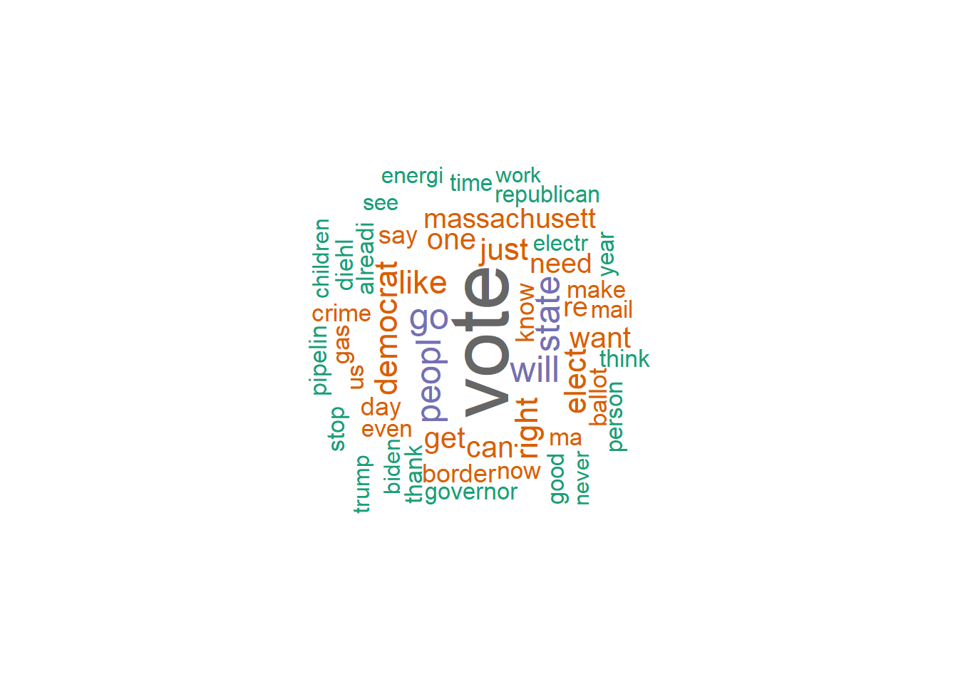

Feature-Occurence Matrix

Code

# DFM that contains hashtags 
Healytag_dfm <- dfm_select(Healy_Dfm, pattern = "#*")
Healytoptag <- names(topfeatures(Healy_Dfm, 30)) 
head(Healytoptag)

[1] "vote"  "will"  "go"    "peopl" "state" "like"

Code

Healytag_fcm <- fcm(Healy_Dfm, context = "document", tri = FALSE)
head(Healytag_fcm)

Feature co-occurrence matrix of: 6 by 334 features.
         features
features  day th best abort protect ma chang two just anyth
  day       3  1    2     1       1  3     1   1    9     1
  th        1  0    1     2       1  2     1   1    1     1
  best      2  1    0     1       2  2     1   1    1     1
  abort     1  2    1     0       1  2     1   1    1     1
  protect   1  1    2     1       4  3     1   1    2     1
  ma        3  2    2     2       3  1     2   3    5     2
[ reached max_nfeat ... 324 more features ]

Semantic Network Visualization

Code

#Visualization of semantic network based on hashtag co-occurrence
Healytopgat_fcm <- fcm_select(Healytag_fcm, pattern = Healytoptag)
textplot_network(Healytopgat_fcm, min_freq = 0.8,
                 omit_isolated = TRUE,
                 edge_color = "#1F78B4",
                 edge_alpha = 0.5,
                 edge_size = 2,
                 vertex_color = "#4D4D4D",
                 vertex_size = 2,
                 vertex_labelcolor = NULL,
                 vertex_labelfont = NULL,
                 vertex_labelsize = 8,
                 offset = NULL)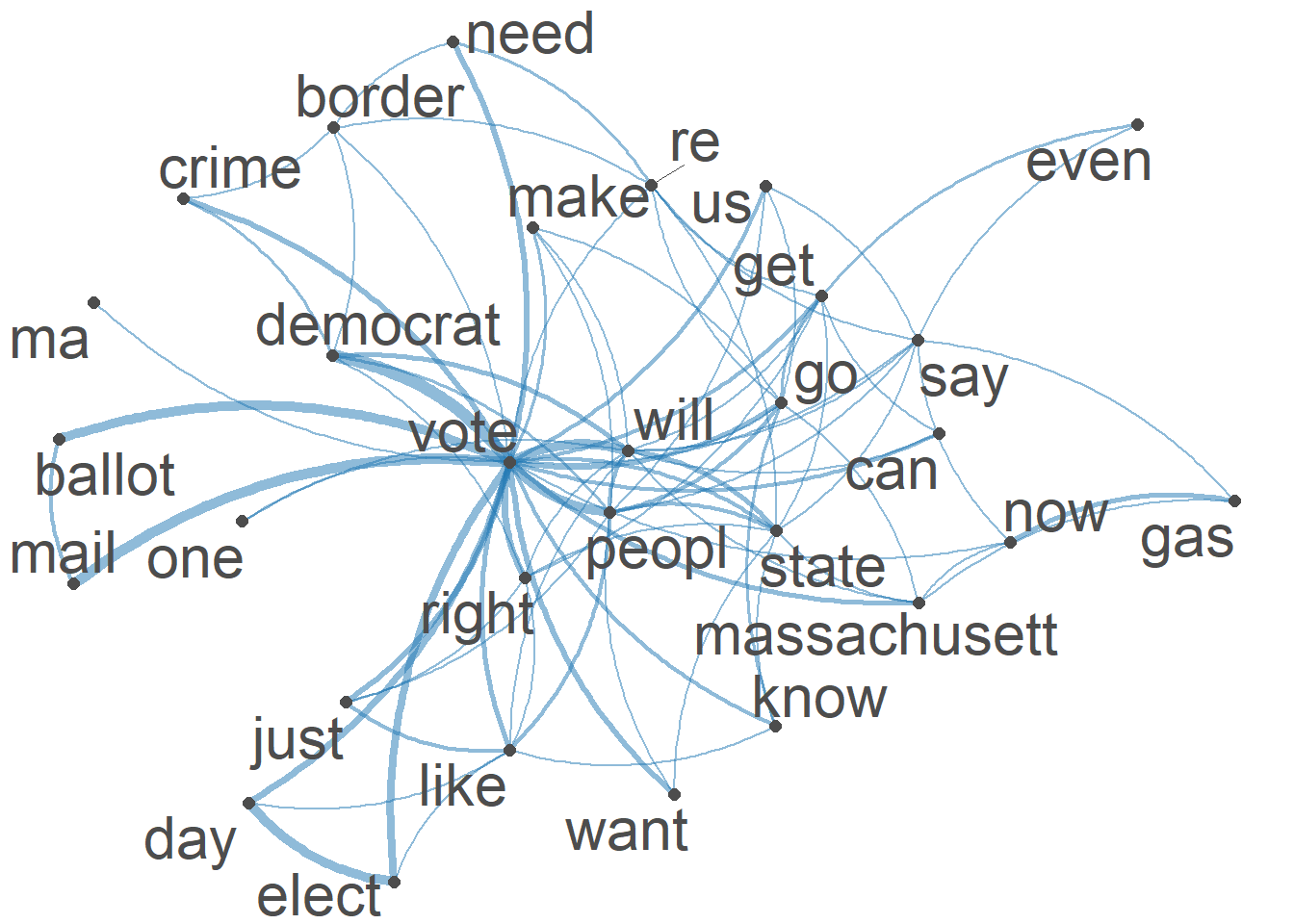

Code

textplot_network(Healytopgat_fcm, vertex_labelsize = 1.5 * rowSums(Healytopgat_fcm)/min(rowSums(Healytopgat_fcm)))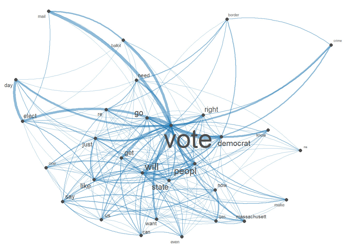

Sentiment Analysis

Code

#convert cleaned Healy_tokens back tp corpus for sentiment analysis
Healy_corpus <- corpus(as.character(Healy_tokens))

NRC Dictionary

Code

# use liwcalike() to estimate sentiment using NRC dictionary
HealyTweetSentiment_nrc <- liwcalike(Healy_corpus, data_dictionary_NRC)
names(HealyTweetSentiment_nrc)

 [1] "docname"      "Segment"      "WPS"          "WC"           "Sixltr"      
 [6] "Dic"          "anger"        "anticipation" "disgust"      "fear"        
[11] "joy"          "negative"     "positive"     "sadness"      "surprise"    
[16] "trust"        "AllPunc"      "Period"       "Comma"        "Colon"       
[21] "SemiC"        "QMark"        "Exclam"       "Dash"         "Quote"       
[26] "Apostro"      "Parenth"      "OtherP"

Code

HealyTweetSentiment_nrc_viz <- HealyTweetSentiment_nrc %>%
  select(c("anger", "anticipation", "disgust", "fear","joy","sadness", "surprise","trust","positive","negative"))

Code

Healy_tr<-data.frame(t(HealyTweetSentiment_nrc_viz)) #transpose

Code

Healy_tr_new <- data.frame(rowSums(Healy_tr[2:1900]))
Healy_tr_mean <- data.frame(rowMeans(Healy_tr[2:1900]))#get mean of sentiment values
names(Healy_tr_new)[1] <- "Count"
Healy_tr_new <- cbind("sentiment" = rownames(Healy_tr_new), Healy_tr_new)
rownames(Healy_tr_new) <- NULL
Healy_tr_new2<-Healy_tr_new[1:8,]

Code

write_csv(Healy_tr_new2,"Healy-Sentiments")
write_csv(Healy_tr_new,"Healy-8 Sentiments")

Code

#Plot One - Count of words associated with each sentiment
quickplot(sentiment, data=Healy_tr_new2, weight=Count, geom="bar", fill=sentiment, ylab="count")+ggtitle("Emotions of REPLIES to Maura Healey Tweets")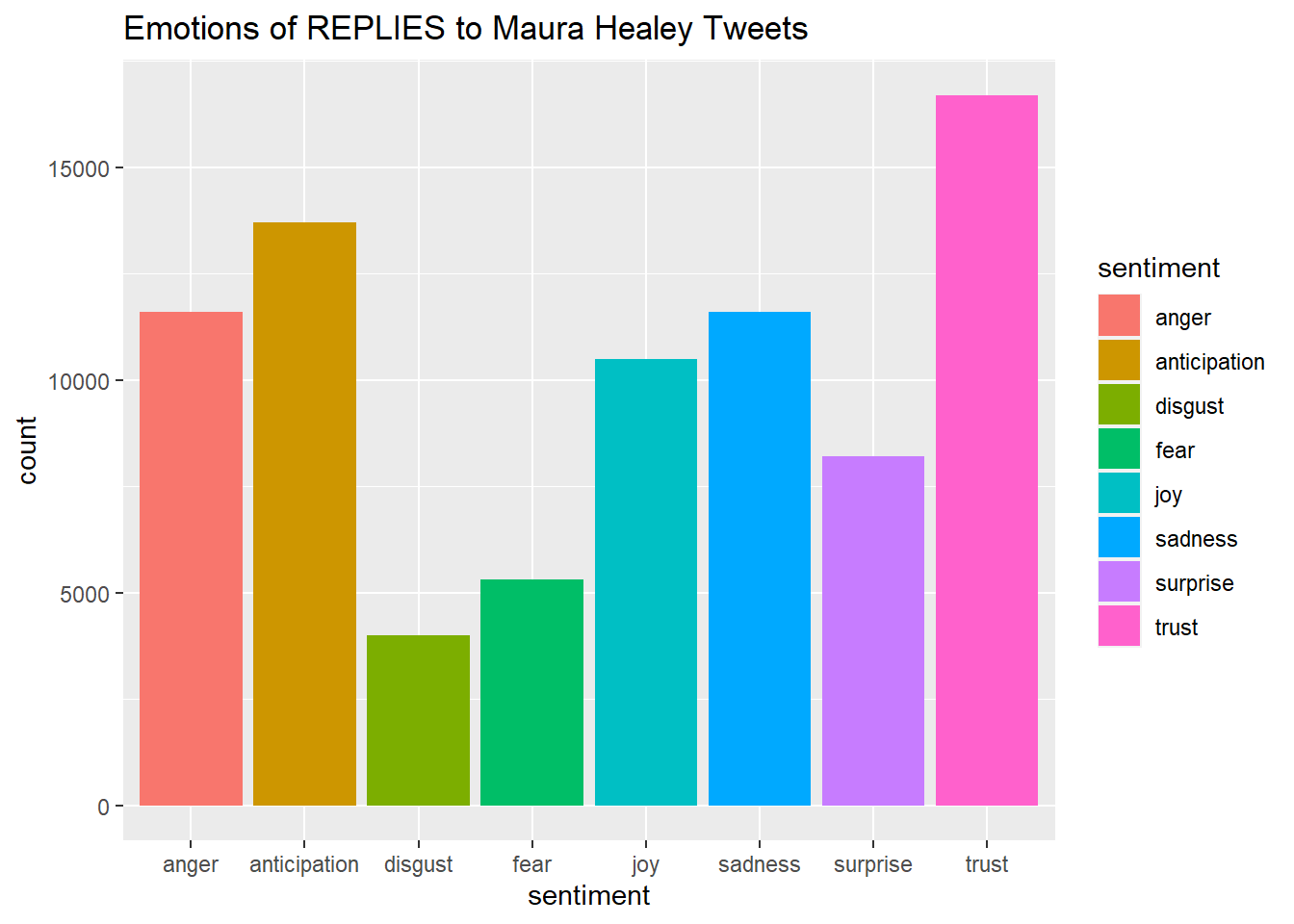

Code

names(Healy_tr_mean)[1] <- "Mean"
Healy_tr_mean <- cbind("sentiment" = rownames(Healy_tr_mean), Healy_tr_mean)
rownames(Healy_tr_mean) <- NULL
Healy_tr_mean2<-Healy_tr_mean[9:10,]
write_csv(Healy_tr_mean2,"Healy-Mean Sentiments")

Code

#Plot One - Count of words associated with each sentiment
quickplot(sentiment, data=Healy_tr_mean2, weight=Mean, geom="bar", fill=sentiment, ylab="Mean Sentiment Score")+ggtitle("Mean Sentiment Scores to Maura Healey Tweets")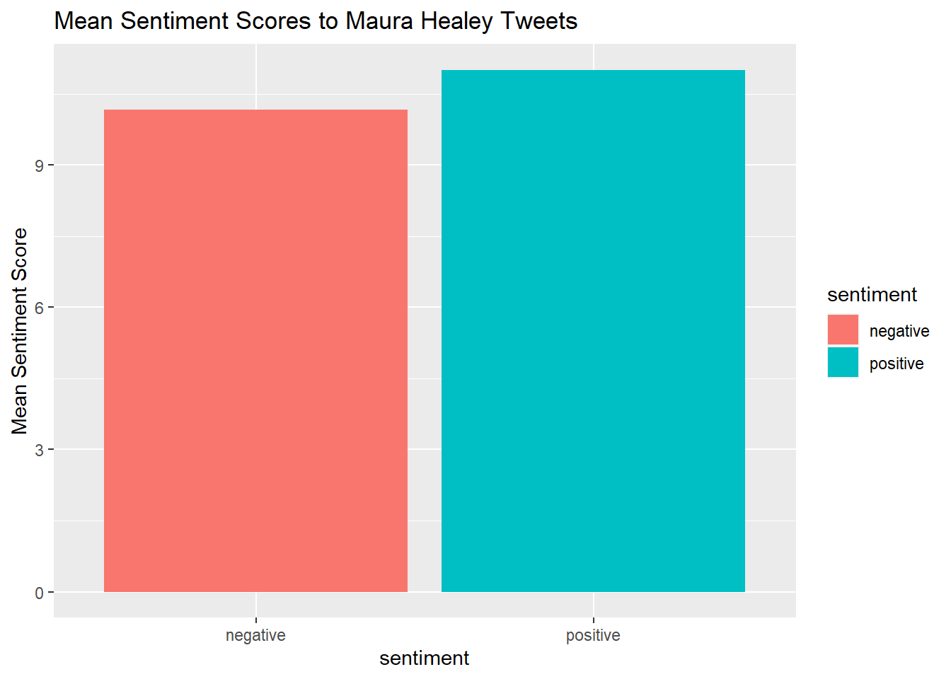

Polarity scores

Code

# POLARITY

Healydf_nrc <- convert(HealyDfm_nrc, to = "data.frame")
names(Healydf_nrc)

 [1] "doc_id"       "anger"        "anticipation" "disgust"      "fear"        
 [6] "joy"          "negative"     "positive"     "sadness"      "surprise"    
[11] "trust"

Code

write_csv(Healydf_nrc,"Healy-Polarity Scores")

Healydf_nrc$polarity <- (Healydf_nrc$positive - Healydf_nrc$negative)/(Healydf_nrc$positive + Healydf_nrc$negative)

Healydf_nrc$polarity[(Healydf_nrc$positive + Healydf_nrc$negative) == 0] <- 0

ggplot(Healydf_nrc) +
  geom_histogram(aes(x=polarity)) +
  theme_bw()

`stat_bin()` using `bins = 30`. Pick better value with `binwidth`.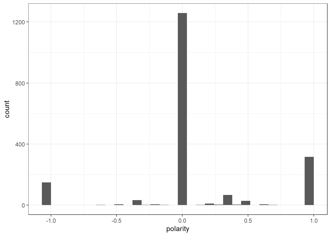

New DF with Polarity scores

Code

Healy_text_df <-as.data.frame(Healy_text_df)
HealyCorpus_Polarity <-as.data.frame((cbind(Healydf_nrc,Healy_text_df)))

New CORPUS (Polarity+text)

Code

HealyCorpus_Polarity <- HealyCorpus_Polarity %>%
    select(c("polarity","Healy_corpus"))

Code

HealyCorpus_Polarity$polarity <- recode(HealyCorpus_Polarity$polarity,
                                      "1" = "positive",
                                      "-1" = "negative",
                                      "0" = "neutral",)

Omit na

Code

HealyCorpus_Polarity <- na.omit(HealyCorpus_Polarity)
head(HealyCorpus_Polarity)

      polarity
text1  neutral
text2 positive
text4  neutral
text6  neutral
text7 negative
text8  neutral
                                                                                                                                                                    Healy_corpus
text1        four days nov th best pitchnnfor starters abortion fully protected ma change two items list just hyperbole anything drive business ma cost energy even higher crazy
text2                                                                                                 reproductive freedom protected ma sent back states… belongs ag understand 
text4                                                                                                                                              preserving democracy come man
text6  like seriously guys republicans fix anything claim able just gonna pull sociallyconservative bs take away right vote alongside social security medicare telegraphing hard
text7                                                                                                                  willing trade democracy lower gas prices will get neither
text8                                                                                                                                                          httpstcopqhknanuo

Convert cleaned DF to corpus

Code

HealyCorpus_P<- corpus(HealyCorpus_Polarity,text_field = "Healy_corpus")

HEALEY- MACHINE LEARNING METHODS

Code

# set seed
set.seed(123)

# create id variable in corpus metadata
docvars(HealyCorpus_P, "id") <- 1:ndoc(HealyCorpus_P)


# create training set (60% of data) and initial test set
N <- ndoc(HealyCorpus_P)
trainIndex <- sample(1:N,.6 * N) 
testIndex <- c(1:N)[-trainIndex]


# split test set in half (so 20% of data are test, 20% of data are held-out)
N <- length(testIndex)
heldOutIndex <- sample(1:N, .5 * N)
testIndex <- testIndex[-heldOutIndex]



# now apply indices to create subsets and dfms
dfmTrain <- corpus_subset(HealyCorpus_P, id %in% trainIndex) %>% tokens() %>% dfm()
dfmTest <- corpus_subset(HealyCorpus_P, id %in% testIndex) %>% tokens() %>% dfm()
dfmHeldOut <- corpus_subset(HealyCorpus_P, id %in% heldOutIndex) %>% tokens() %>% dfm()


head(trainIndex)

[1] 415 463 179 526 195 938

Code

head(testIndex)

[1]  3  4 12 14 15 20

NB model

Code

polarity_NaiveBayes <- textmodel_nb(dfmTrain, docvars(dfmTrain, "polarity"), distribution = "Bernoulli") 
summary(polarity_NaiveBayes)


Call:
textmodel_nb.dfm(x = dfmTrain, y = docvars(dfmTrain, "polarity"), 
    distribution = "Bernoulli")

Class Priors:
(showing first 3 elements)
negative  neutral positive 
  0.3333   0.3333   0.3333 

Estimated Feature Scores:
         reproductive  freedom protected      ma     sent     back   states
negative     0.011494 0.011494  0.011494 0.04598 0.011494 0.022989 0.011494
neutral      0.001309 0.003927  0.001309 0.02618 0.002618 0.006545 0.003927
positive     0.010582 0.015873  0.015873 0.04233 0.015873 0.037037 0.015873
               …  belongs       ag understand  willing    trade democracy
negative 0.02299 0.011494 0.011494   0.011494 0.022989 0.022989  0.022989
neutral  0.02225 0.001309 0.006545   0.001309 0.002618 0.001309  0.002618
positive 0.01587 0.010582 0.031746   0.010582 0.005291 0.005291  0.015873
            lower     gas   prices    will     get  neither httpstcopqhknanuo
negative 0.034483 0.02299 0.057471 0.09195 0.04598 0.022989          0.011494
neutral  0.002618 0.01702 0.003927 0.04188 0.03272 0.001309          0.002618
positive 0.005291 0.06878 0.010582 0.06878 0.06349 0.010582          0.005291
            build  economy    works everyone  raising   living     cost
negative 0.022989 0.022989 0.022989 0.022989 0.022989 0.022989 0.022989
neutral  0.001309 0.002618 0.001309 0.006545 0.001309 0.002618 0.003927
positive 0.010582 0.015873 0.005291 0.005291 0.015873 0.010582 0.015873
            taxes  chasing
negative 0.045977 0.022989
neutral  0.006545 0.001309
positive 0.005291 0.005291

Code

dfmTestMatched <- dfm_match(dfmTest, features = featnames(dfmTrain))

CONFUSION MATRIX

Code

# create a confusion matrix 
actual <- docvars(dfmTestMatched, "polarity")
predicted <- predict(polarity_NaiveBayes, newdata = dfmTestMatched)
confusion <- table(actual, predicted)

# now calculate a number of statistics related to the confusion matrix
confusionMatrix(confusion, mode = "everything")

Confusion Matrix and Statistics

          predicted
actual     negative neutral positive
  negative        2      33        1
  neutral         0     240        3
  positive        0      58        8

Overall Statistics
                                          
               Accuracy : 0.7246          
                 95% CI : (0.6743, 0.7711)
    No Information Rate : 0.9594          
    P-Value [Acc > NIR] : 1               
                                          
                  Kappa : 0.1313          
                                          
 Mcnemar's Test P-Value : <2e-16          

Statistics by Class:

                     Class: negative Class: neutral Class: positive
Sensitivity                 1.000000         0.7251         0.66667
Specificity                 0.900875         0.7857         0.82583
Pos Pred Value              0.055556         0.9877         0.12121
Neg Pred Value              1.000000         0.1078         0.98566
Precision                   0.055556         0.9877         0.12121
Recall                      1.000000         0.7251         0.66667
F1                          0.105263         0.8362         0.20513
Prevalence                  0.005797         0.9594         0.03478
Detection Rate              0.005797         0.6957         0.02319
Detection Prevalence        0.104348         0.7043         0.19130
Balanced Accuracy           0.950437         0.7554         0.74625

Code

predicted_prob <- predict(polarity_NaiveBayes, newdata = dfmTestMatched, type = "probability")
head(predicted_prob)

           negative   neutral     positive
text4  8.369084e-14 1.0000000 4.927139e-08
text6  1.084335e-08 0.9999950 4.980505e-06
text14 1.244174e-11 0.9999826 1.737715e-05
text17 6.671955e-13 0.9999999 9.920512e-08
text18 9.471524e-15 1.0000000 3.598392e-08
text24 2.010070e-12 1.0000000 3.591003e-08

Code

summary(predicted_prob)

    negative           neutral          positive       
 Min.   :0.000000   Min.   :0.0000   Min.   :0.00e+00  
 1st Qu.:0.000000   1st Qu.:1.0000   1st Qu.:0.00e+00  
 Median :0.000000   Median :1.0000   Median :3.00e-07  
 Mean   :0.005803   Mean   :0.9541   Mean   :4.01e-02  
 3rd Qu.:0.000000   3rd Qu.:1.0000   3rd Qu.:1.33e-05  
 Max.   :1.000000   Max.   :1.0000   Max.   :1.00e+00

Code

# The most positive review
mostPos <- sort.list(predicted_prob[,1], dec=F)[1]
as.character(corpus_subset(HealyCorpus_P, id %in% testIndex))[mostPos]

              text1320 
" casting vote modern"

Code

mostNeg <- sort.list(predicted_prob[,1], dec=T)[1]
as.character(corpus_subset(HealyCorpus_P, id %in% testIndex))[mostNeg]

                                                                                                                                                                        text903 
" black poverty charts dem areann  africanamerican households boston live poverty line statistic conceals huge inequities across neighborhoods ranging  hyde park  charlestown"

Code

# The most positive review
mixed <- sort.list(abs(predicted_prob[,1] - .5), dec=F)[1]
predicted_prob[mixed,]

  negative    neutral   positive 
0.00135779 0.29476010 0.70388211

Code

as.character(corpus_subset(HealyCorpus_P, id %in% testIndex))[mixed]

                                                                                                                                                                                     text1194 
" gemini  omg almost east coast california speak especially witch becomes gov thing holding together balance r gov entire legislature d unliked many reluctance ban covid 🗥 kids pissed moms"

Naive Bayes -held out

Code

actual <- docvars(dfmHeldOut)$polarity
count(actual)

         x freq
1 negative   23
2  neutral  256
3 positive   66

Code

dfmHeldOutMatched <- dfm_match(dfmHeldOut, features = featnames(dfmTrain))
predicted.nb <- predict(polarity_NaiveBayes, dfmHeldOutMatched)
count(predicted.nb)

         x freq
1 negative    1
2  neutral  320
3 positive   24

Code

confusion <- table(actual, predicted.nb)
confusionMatrix(confusion, mode = "everything")

Confusion Matrix and Statistics

          predicted.nb
actual     negative neutral positive
  negative        1      22        0
  neutral         0     254        2
  positive        0      44       22

Overall Statistics
                                          
               Accuracy : 0.8029          
                 95% CI : (0.7569, 0.8436)
    No Information Rate : 0.9275          
    P-Value [Acc > NIR] : 1               
                                          
                  Kappa : 0.3391          
                                          
 Mcnemar's Test P-Value : NA              

Statistics by Class:

                     Class: negative Class: neutral Class: positive
Sensitivity                 1.000000         0.7937         0.91667
Specificity                 0.936047         0.9200         0.86293
Pos Pred Value              0.043478         0.9922         0.33333
Neg Pred Value              1.000000         0.2584         0.99283
Precision                   0.043478         0.9922         0.33333
Recall                      1.000000         0.7937         0.91667
F1                          0.083333         0.8819         0.48889
Prevalence                  0.002899         0.9275         0.06957
Detection Rate              0.002899         0.7362         0.06377
Detection Prevalence        0.066667         0.7420         0.19130
Balanced Accuracy           0.968023         0.8569         0.88980

SVM

Code

# set seed
set.seed(123)

# set of training data
newTrainIndex <- trainIndex[sample(1:length(trainIndex))]

# create small DFM
dfmTrainSmall <- corpus_subset(HealyCorpus_P, id %in% newTrainIndex) %>% dfm(remove = stopwords("English"), remove_punct=T)

# trim the DFM down to frequent terms
dfmTrainSmall <- dfm_trim(dfmTrainSmall, min_docfreq = 20, min_termfreq = 20)

dim(dfmTrainSmall)

[1] 1034   34

Code

# run model
polarity_SVM <- textmodel_svm(dfmTrainSmall, docvars(dfmTrainSmall, "polarity")) 

# update test set
dfmTestMatchedSmall <- dfm_match(dfmTest, features = featnames(dfmTrainSmall))

# create a confusion matrix 
actual <- docvars(dfmTestMatchedSmall, "polarity")
predicted <- predict(polarity_SVM, newdata = dfmTestMatchedSmall)
confusion <- table(actual, predicted)

Confusion Matrix

Code

# now calculate a number of statistics related to the confusion matrix
confusionMatrix(confusion, mode = "everything")

Confusion Matrix and Statistics

          predicted
actual     negative neutral positive
  negative        2      32        2
  neutral         0     240        3
  positive        0      53       13

Overall Statistics
                                          
               Accuracy : 0.7391          
                 95% CI : (0.6894, 0.7847)
    No Information Rate : 0.942           
    P-Value [Acc > NIR] : 1               
                                          
                  Kappa : 0.1995          
                                          
 Mcnemar's Test P-Value : <2e-16          

Statistics by Class:

                     Class: negative Class: neutral Class: positive
Sensitivity                 1.000000         0.7385         0.72222
Specificity                 0.900875         0.8500         0.83792
Pos Pred Value              0.055556         0.9877         0.19697
Neg Pred Value              1.000000         0.1667         0.98208
Precision                   0.055556         0.9877         0.19697
Recall                      1.000000         0.7385         0.72222
F1                          0.105263         0.8451         0.30952
Prevalence                  0.005797         0.9420         0.05217
Detection Rate              0.005797         0.6957         0.03768
Detection Prevalence        0.104348         0.7043         0.19130
Balanced Accuracy           0.950437         0.7942         0.78007

Code

# check code---Error in order(V1) : object 'V1' not found
svmCoefs <- as.data.frame(t(coefficients(polarity_SVM)))
head(svmCoefs,10)

            positive    negative     neutral
ma        0.10642383  0.04095159 -0.15027369
gas       0.63259122 -0.23232753 -0.45305789
will     -0.04905536  0.17855470 -0.11240942
get       0.13327219 -0.08977719 -0.04335252
state     0.32094424 -0.03608965 -0.28125136
governor -0.23191741  0.03187021  0.19601274
re        0.19742408  0.07659889 -0.25219334
just     -0.11477470  0.03795018  0.06346217
one       0.36764128 -0.05616672 -0.31978665
biden     0.20245429 -0.46449151  0.02273121

Code

tail(svmCoefs,10)

            positive    negative     neutral
go       -0.30889746 -0.06202332  0.34283740
need      0.08641445 -0.01586162 -0.07350022
now       0.12340404  0.19171685 -0.26537615
want     -0.08106290  0.21969589 -0.12917587
know      0.44976743  0.01858271 -0.47835868
us        0.06998385 -0.06974139 -0.01704071
election  1.45926123 -0.33623228 -1.30718337
already  -0.19044299 -0.02657631  0.21397132
border    0.30428331 -0.08398931 -0.24725324
Bias     -0.73363968 -0.84683933  0.58081363

RANDOM FOREST

Code

library(randomForest)

Error in library(randomForest): there is no package called 'randomForest'

Code

dfmTrainSmallRf <- convert(dfmTrainSmall, to = "matrix")
dfmTestMatchedSmallRf <- convert(dfmTestMatchedSmall, to = "matrix")

set.seed(123)
Healey_polarity_RF <- randomForest(dfmTrainSmallRf, 
                            y = as.factor(docvars(dfmTrainSmall)$polarity),
                            xtest = dfmTestMatchedSmallRf, 
                            ytest = as.factor(docvars(dfmTestMatchedSmall)$polarity),
                            importance = TRUE,
                            mtry = 20,
                            ntree = 100
)

Error in randomForest(dfmTrainSmallRf, y = as.factor(docvars(dfmTrainSmall)$polarity), : could not find function "randomForest"

Confusion Matrix

Code

actual <- as.factor(docvars(dfmTestMatchedSmall)$polarity)
predicted <- Healey_polarity_RF$test[['predicted']]

Error in eval(expr, envir, enclos): object 'Healey_polarity_RF' not found

Code

confusion <- table(actual,predicted)
confusionMatrix(confusion, mode="everything")

Confusion Matrix and Statistics

          predicted
actual     negative neutral positive
  negative        2      32        2
  neutral         0     240        3
  positive        0      53       13

Overall Statistics
                                          
               Accuracy : 0.7391          
                 95% CI : (0.6894, 0.7847)
    No Information Rate : 0.942           
    P-Value [Acc > NIR] : 1               
                                          
                  Kappa : 0.1995          
                                          
 Mcnemar's Test P-Value : <2e-16          

Statistics by Class:

                     Class: negative Class: neutral Class: positive
Sensitivity                 1.000000         0.7385         0.72222
Specificity                 0.900875         0.8500         0.83792
Pos Pred Value              0.055556         0.9877         0.19697
Neg Pred Value              1.000000         0.1667         0.98208
Precision                   0.055556         0.9877         0.19697
Recall                      1.000000         0.7385         0.72222
F1                          0.105263         0.8451         0.30952
Prevalence                  0.005797         0.9420         0.05217
Detection Rate              0.005797         0.6957         0.03768
Detection Prevalence        0.104348         0.7043         0.19130
Balanced Accuracy           0.950437         0.7942         0.78007

Code

varImpPlot(Healey_polarity_RF)

Error in varImpPlot(Healey_polarity_RF): could not find function "varImpPlot"

DIEHL DATA

Load Data

Code

Diehl <- read_csv("Diehl.csv")

Rows: 497 Columns: 79
── Column specification ────────────────────────────────────────────────────────
Delimiter: ","
chr  (34): edit_history_tweet_ids, text, lang, source, reply_settings, entit...
dbl  (18): id, conversation_id, referenced_tweets.replied_to.id, referenced_...
lgl  (23): referenced_tweets.retweeted.id, edit_controls.is_edit_eligible, r...
dttm  (4): edit_controls.editable_until, created_at, author.created_at, __tw...

ℹ Use `spec()` to retrieve the full column specification for this data.
ℹ Specify the column types or set `show_col_types = FALSE` to quiet this message.

Code

Diehl$text <- gsub("@[[:alpha:]]*","", Diehl$text) #remove Twitter handles
Diehl$text <- gsub("&amp", "", Diehl$text)
Diehl$text <- gsub("_", "", Diehl$text)

Data Cleaning/ Preprocessing

Code

Diehl_corpus <- Corpus(VectorSource(Diehl$text))
Diehl_corpus <- tm_map(Diehl_corpus, tolower) #lowercase
Diehl_corpus <- tm_map(Diehl_corpus, removeWords, 
                       c("s","geoff", "diehl","rt", "amp"))
Diehl_corpus <- tm_map(Diehl_corpus, removeWords, 
                       stopwords("english"))
Diehl_corpus <- tm_map(Diehl_corpus, removePunctuation)
Diehl_corpus <- tm_map(Diehl_corpus, stripWhitespace)
Diehl_corpus <- tm_map(Diehl_corpus, removeNumbers)

Diehl_corpus <- corpus(Diehl_corpus,text_field = "text") 

Diehl_text_df <- as.data.frame(Diehl_corpus)

Tokenize and stemming

Code

Diehl_tokens <- tokens(Diehl_corpus)
Diehl_tokens <- tokens_wordstem(Diehl_tokens)
print(Diehl_tokens)

Tokens consisting of 497 documents.
text1 :
[1] "still"   "beat"    "fascism" "day"     "week"    "📴"     

text2 :
[1] "wear" "mask" "'"    "re"   "dumb"

text3 :
 [1] "'"       "mention" "mask"    "pay"     "compani" "can"     "charg"  
 [8] "whatev"  "want"    "follow"  "'"       "ll"     
[ ... and 10 more ]

text4 :
 [1] "argument" "gas"      "pipelin"  "energi"   "independ" "right"   
 [7] "now"      "new"      "england"  "get"      "lng"      "deliveri"
[ ... and 18 more ]

text5 :
 [1] "shit"     "u"        "dumb"     "masker"   "democrat" "still"   
 [7] "fuck"     "everyon"  "caus"     "price"    "hike"     "higher"  
[ ... and 7 more ]

text6 :
 [1] "compani"  "take"     "profit"   "loss"     "kinder"   "morgan"  
 [7] "elect"    "need"     "proof"    "energi"   "independ" "way"     
[ ... and 7 more ]

[ reached max_ndoc ... 491 more documents ]

Code

dfm(Diehl_tokens)

Document-feature matrix of: 497 documents, 1,921 features (99.49% sparse) and 0 docvars.
       features
docs    still beat fascism day week📴 wear mask ' re
  text1     1    1       1   1    1 1    0    0 0  0
  text2     0    0       0   0    0 0    1    1 1  1
  text3     0    0       0   0    0 0    0    1 2  0
  text4     0    0       0   0    0 0    0    0 0  0
  text5     1    0       0   0    0 0    0    0 0  0
  text6     0    0       0   0    0 0    0    0 0  0
[ reached max_ndoc ... 491 more documents, reached max_nfeat ... 1,911 more features ]

Create dfm

Code

# create a full dfm for comparison---use this to append to polarity
Diehl_Dfm <- tokens(Diehl_tokens,
                    remove_punct = TRUE,
                    remove_symbols = TRUE,
                    remove_numbers = TRUE,
                    remove_url = TRUE,
                    split_hyphens = FALSE,
                    split_tags = FALSE,
                    include_docvars = TRUE) %>%
  tokens_tolower() %>%
  dfm(remove = stopwords('english')) %>%
  dfm_trim(min_termfreq = 10, verbose = FALSE) %>%
  dfm()

TF-IDF

Code

topfeatures(Diehl_Dfm)

  vote school     go   like   will    get healey public   know   just 
    57     54     47     43     43     39     39     35     32     32

Code

Diehl_tf_dfm <- dfm_tfidf(Diehl_Dfm, force = TRUE) #create a new DFM by tf-idf scores
topfeatures(Diehl_tf_dfm) ## this shows top words by tf-idf

  school     vote       go     like     will      get   healey   public 
61.56291 55.88012 50.43603 46.14361 46.14361 44.46210 44.46210 43.18854 
    know     just 
39.97435 39.48667

Code

# convert corpus to dfm using the dictionary---use to append 
DiehlDfm_nrc <- tokens(Diehl_tokens,
                       remove_punct = TRUE,
                       remove_symbols = TRUE,
                       remove_numbers = TRUE,
                       remove_url = TRUE,
                       split_tags = FALSE,
                       split_hyphens = FALSE,
                       include_docvars = TRUE) %>%
  tokens_tolower() %>%
  dfm(remove = stopwords('english')) %>%
  dfm_trim(min_termfreq = 10, verbose = FALSE) %>%
  dfm() %>%
  dfm_lookup(data_dictionary_NRC)


dim(DiehlDfm_nrc)

[1] 497  10

Code

head(DiehlDfm_nrc, 10)

Document-feature matrix of: 10 documents, 10 features (70.00% sparse) and 0 docvars.
       features
docs    anger anticipation disgust fear joy negative positive sadness surprise
  text1     0            0       0    0   0        0        0       0        0
  text2     0            0       0    0   0        0        0       0        0
  text3     1            1       0    0   1        1        1       1        1
  text4     1            3       0    0   1        0        3       0        1
  text5     0            0       0    0   0        0        0       0        0
  text6     0            0       0    0   0        0        1       0        0
       features
docs    trust
  text1     0
  text2     0
  text3     1
  text4     1
  text5     0
  text6     1
[ reached max_ndoc ... 4 more documents ]

Word CLoud

Code

library(RColorBrewer)
textplot_wordcloud(Diehl_Dfm, scale=c(5,1), max.words=50, random.order=FALSE, rot.per=0.35, use.r.layout=FALSE, colors=brewer.pal(8, "Dark2"))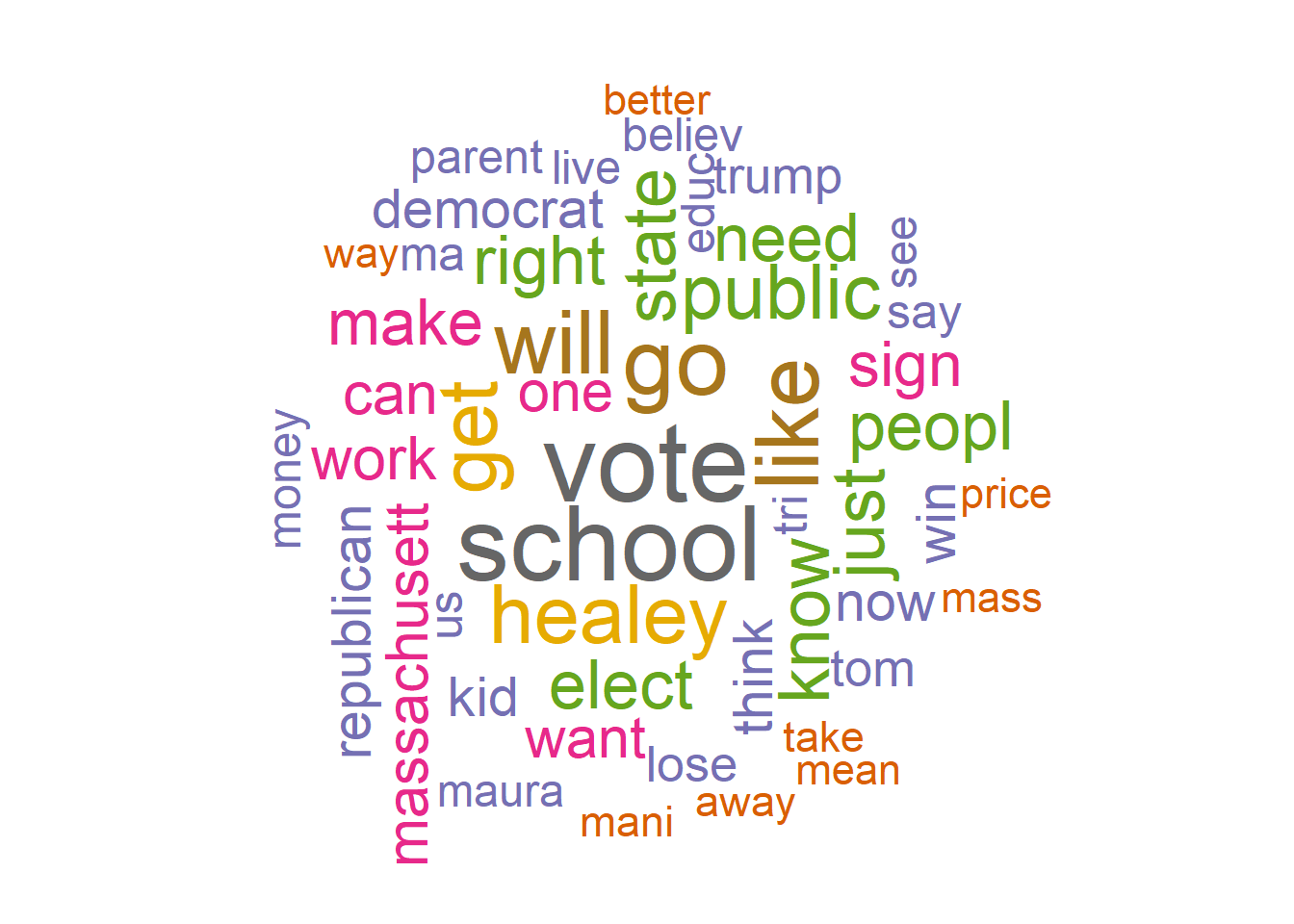

Feature-occurrence matrix

Code

Diehltag_dfm <- dfm_select(Diehl_Dfm, pattern = "#*")
Diehltoptag <- names(topfeatures(Diehl_Dfm, 30)) 
head(Diehltoptag)

[1] "vote"   "school" "go"     "like"   "will"   "get"

Code

Diehltag_fcm <- fcm(Diehl_Dfm)
head(Diehltag_fcm)

Feature co-occurrence matrix of: 6 by 74 features.
        features
features re can want see vote like gas energi right now
    re    1   0    2   0    0    1   0      1     4   0
    can   0   1    3   1    5    3   2      2     2   2
    want  0   0    4   1    2    3   0      0     4   3
    see   0   0    0   1    5    3   0      0     0   0
    vote  0   0    0   0    5    4   1      1     1   2
    like  0   0    0   0    0    1   1      1     2   3
[ reached max_nfeat ... 64 more features ]

Semantic Network Analysis

Code

#Visualization of semantic network based on hashtag co-occurrence

Diehltopgat_fcm <- fcm_select(Diehltag_fcm, pattern = Diehltoptag)
textplot_network(Diehltopgat_fcm, min_freq = 0.8,
                 omit_isolated = TRUE,
                 edge_color = "#1F78B4",
                 edge_alpha = 0.5,
                 edge_size = 2,
                 vertex_color = "#4D4D4D",
                 vertex_size = 2,
                 vertex_labelcolor = NULL,
                 vertex_labelfont = NULL,
                 vertex_labelsize = 8,
                 offset = NULL)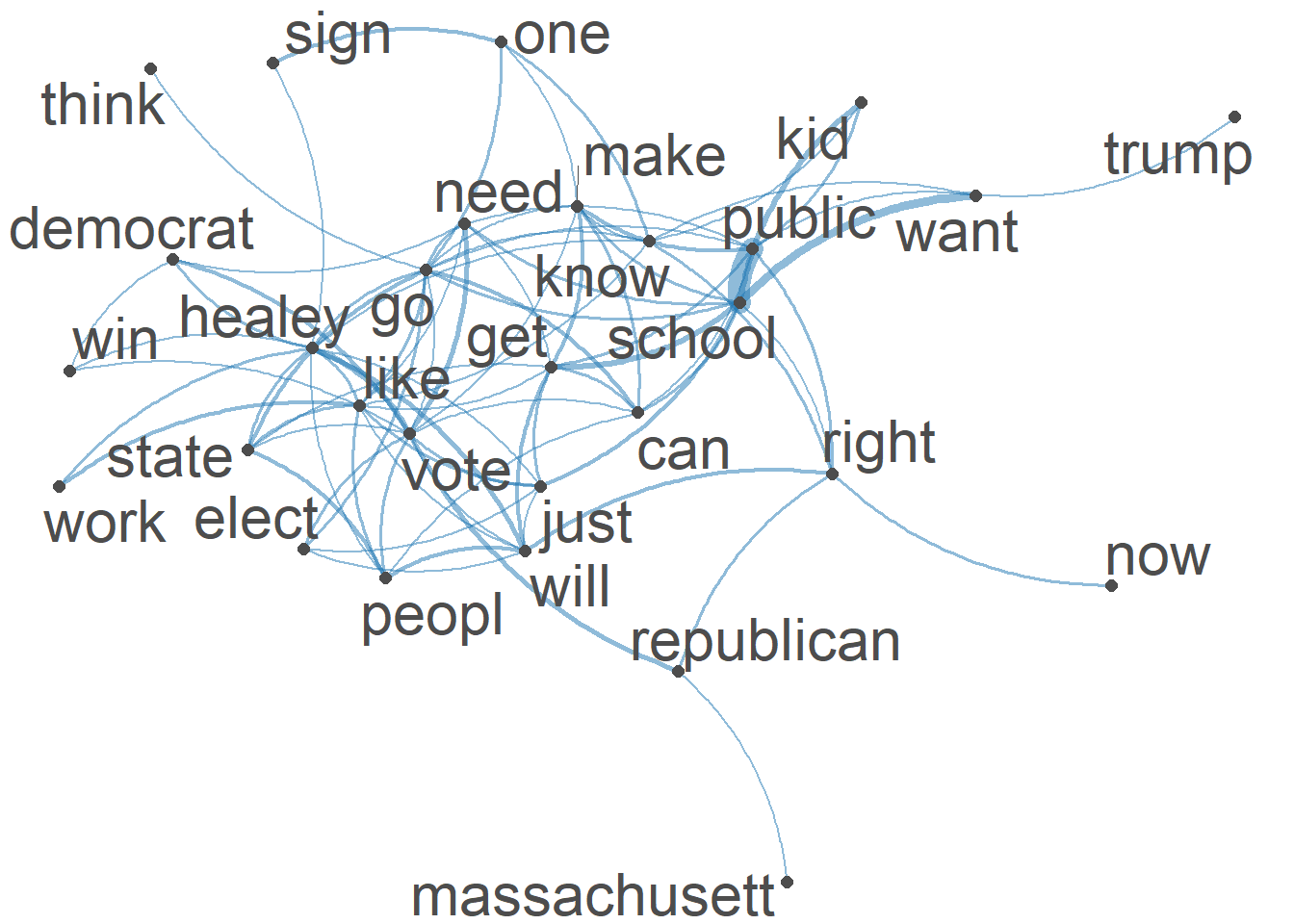

Sentiment Analysis

NRC Dictionary

Code

#convert cleaned Diehl_tokens back tp corpus for sentiment analysis
Diehl_corpus <- corpus(as.character(Diehl_tokens))

# use liwcalike() to estimate sentiment using NRC dictionary
DiehlTweetSentiment_nrc <- liwcalike(Diehl_corpus, data_dictionary_NRC)

names(DiehlTweetSentiment_nrc)

 [1] "docname"      "Segment"      "WPS"          "WC"           "Sixltr"      
 [6] "Dic"          "anger"        "anticipation" "disgust"      "fear"        
[11] "joy"          "negative"     "positive"     "sadness"      "surprise"    
[16] "trust"        "AllPunc"      "Period"       "Comma"        "Colon"       
[21] "SemiC"        "QMark"        "Exclam"       "Dash"         "Quote"       
[26] "Apostro"      "Parenth"      "OtherP"

Code

DiehlTweetSentiment_nrc_viz <- DiehlTweetSentiment_nrc %>%
  select(c("anger", "anticipation", "disgust", "fear","joy","sadness", "surprise","trust","positive","negative"))


Diehl_tr<-data.frame(t(DiehlTweetSentiment_nrc_viz)) #transpose

Diehl_tr_new <- data.frame(rowSums(Diehl_tr[2:497]))
Diehl_tr_mean <- data.frame(rowMeans(Diehl_tr[2:497]))#get mean of sentiment values
names(Diehl_tr_new)[1] <- "Count"
Diehl_tr_new <- cbind("sentiment" = rownames(Diehl_tr_new), Diehl_tr_new)
rownames(Diehl_tr_new) <- NULL
Diehl_tr_new2<-Diehl_tr_new[1:8,]
write_csv(Diehl_tr_new2,"Diehl- 8 Sentiments")

Code

#Plot One - Count of words associated with each sentiment
quickplot(sentiment, data=Diehl_tr_new2, weight=Count, geom="bar", fill=sentiment, ylab="count")+ggtitle("Emotions to REPLIES Geoff Diehl Tweets")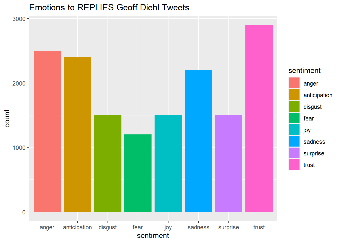

Code

names(Diehl_tr_mean)[1] <- "Mean"
Diehl_tr_mean <- cbind("sentiment" = rownames(Diehl_tr_mean), Diehl_tr_mean)
rownames(Diehl_tr_mean) <- NULL
Diehl_tr_mean2<-Diehl_tr_mean[9:10,]
write_csv(Diehl_tr_mean2,"Diehl -Mean Sentiments")

Code

#Plot One - Count of words associated with each sentiment
quickplot(sentiment, data=Diehl_tr_mean2, weight=Mean, geom="bar", fill=sentiment, ylab="Mean Sentiment Score")+ggtitle("Mean Sentiment Scores to Geoff Diehl Tweets")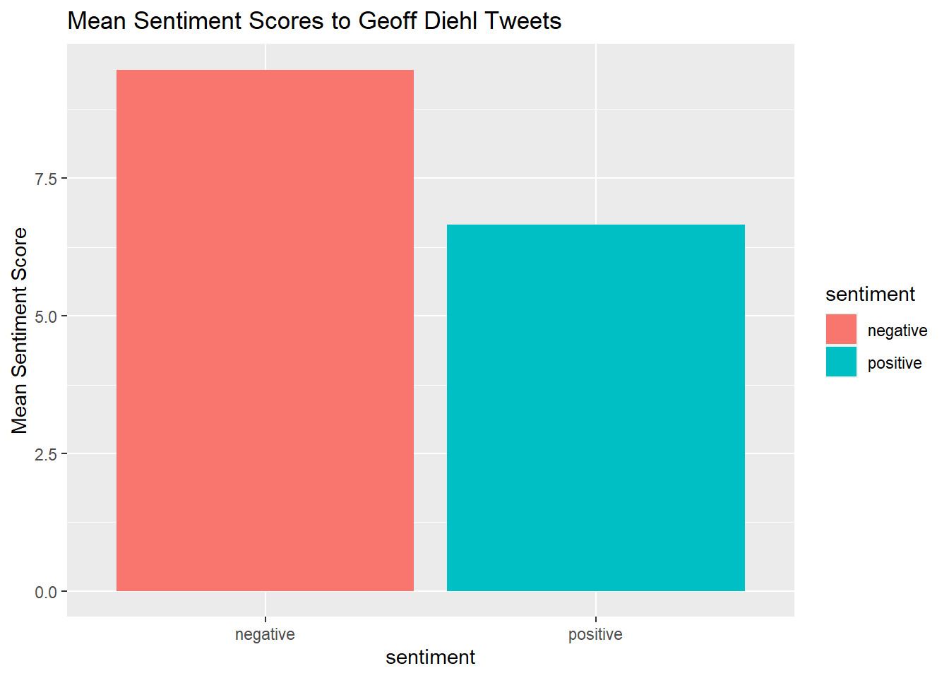

Polarity Scores

Code

Diehldf_nrc <- convert(DiehlDfm_nrc, to = "data.frame")
write_csv(Diehldf_nrc, "Diehl- Polarity Scores")

Diehldf_nrc$polarity <- (Diehldf_nrc$positive - Diehldf_nrc$negative)/(Diehldf_nrc$positive + Diehldf_nrc$negative)

Diehldf_nrc$polarity[(Diehldf_nrc$positive + Diehldf_nrc$negative) == 0] <- 0

ggplot(Diehldf_nrc) +
  geom_histogram(aes(x=polarity)) +
  theme_bw()

`stat_bin()` using `bins = 30`. Pick better value with `binwidth`.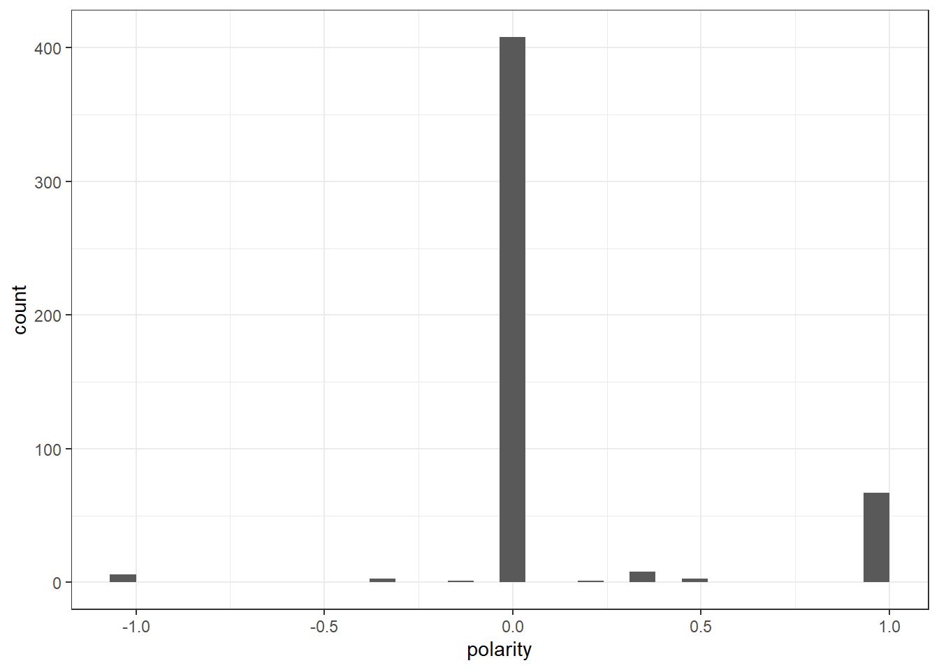

Bind to new DF

Code

Diehl_text_df <-as.data.frame(Diehl_text_df)
DiehlCorpus_Polarity <-as.data.frame((cbind(Diehldf_nrc,Diehl_text_df)))

subset to polarity and text

Code

DiehlCorpus_Polarity <- DiehlCorpus_Polarity %>%
  select(c("polarity","Diehl_corpus"))


DiehlCorpus_Polarity$polarity <- recode(DiehlCorpus_Polarity$polarity,
                                        "1" = "positive",
                                        "-1" = "negative",
                                        "0" = "neutral",)

Cleaned DF

Code

DiehlCorpus_Polarity <- na.omit(DiehlCorpus_Polarity)
head(DiehlCorpus_Polarity)

      polarity
text1  neutral
text2  neutral
text3  neutral
text4 positive
text5  neutral
text6 positive
                                                                                                                                                                                                                  Diehl_corpus
text1                                                                                                                                                                                           still beats fascism day week 📴
text2                                                                                                                                                                                                       wear mask ’re dumb
text3                                                                                     ’ mentioning masks paying companies can charge whatever want follow ’ll see shareholders companies keep voting party like dumb poor…
text4  argument gas pipelines energy independence right now new england gets lng deliveries international shipments nthese corporations making profit another story vg blckrck use public funds turn profit pull public money 
text5                                                                                                         shit u dumb masker democrats still fucked everyone caused price hikes higher taxes fn maskers u don’t know squat
text6                                                                     companies take profit loss kinder morgan elected need proof energy independence way actually take control prices give billionaires httpstcodairdldph

New Corpus with polarity scores

Code

DiehlCorpus_P<- corpus(DiehlCorpus_Polarity,text_field = "Diehl_corpus")

DIEHL-MACHINE LEARNING

Code

# set seed
set.seed(123)

# create id variable in corpus metadata
docvars(DiehlCorpus_P, "id") <- 1:ndoc(DiehlCorpus_P)


# create training set (60% of data) and initial test set
DN <- ndoc(DiehlCorpus_P)
DtrainIndex <- sample(1:DN,.6 * DN) 
DtestIndex <- c(1:N)[-DtrainIndex]


# split test set in half (so 20% of data are test, 20% of data are held-out)
DN <- length(DtestIndex)
DheldOutIndex <- sample(1:DN, .5 * DN)
DtestIndex <- DtestIndex[-DheldOutIndex]



# now apply indices to create subsets and dfms
DdfmTrain <- corpus_subset(DiehlCorpus_P, id %in% DtrainIndex) %>% tokens() %>% dfm()
DdfmTest <- corpus_subset(DiehlCorpus_P, id %in% DtestIndex) %>% tokens() %>% dfm()
DdfmHeldOut <- corpus_subset(DiehlCorpus_P, id %in% DheldOutIndex) %>% tokens() %>% dfm()


head(DtrainIndex)

[1] 415 463 179  14 195 426

Code

head(DtestIndex)

[1]  1  3  6  8  9 15

NB model

Code

polarity_NaiveBayes <- textmodel_nb(DdfmTrain, docvars(DdfmTrain, "polarity"), distribution = "Bernoulli") 
summary(polarity_NaiveBayes)


Call:
textmodel_nb.dfm(x = DdfmTrain, y = docvars(DdfmTrain, "polarity"), 
    distribution = "Bernoulli")

Class Priors:
(showing first 3 elements)
negative  neutral positive 
  0.3333   0.3333   0.3333 

Estimated Feature Scores:
             wear     mask      '      re    dumb argument     gas pipelines
negative 0.142857 0.142857 0.4286 0.14286 0.14286 0.142857 0.14286   0.14286
neutral  0.008163 0.008163 0.1347 0.02857 0.02041 0.008163 0.02041   0.02449
positive 0.023810 0.023810 0.1667 0.04762 0.02381 0.071429 0.09524   0.04762
          energy independence   right     now     new  england     gets
negative 0.14286     0.142857 0.14286 0.28571 0.14286 0.142857 0.142857
neutral  0.02449     0.008163 0.02449 0.03265 0.01633 0.004082 0.004082
positive 0.07143     0.047619 0.11905 0.11905 0.11905 0.047619 0.095238
              lng deliveries international shipments   nthese corporations
negative 0.142857   0.142857      0.142857  0.142857 0.142857     0.142857
neutral  0.004082   0.004082      0.004082  0.004082 0.004082     0.008163
positive 0.047619   0.047619      0.047619  0.047619 0.047619     0.047619
          making   profit another    story       vg  blckrck      use   public
negative 0.14286 0.142857 0.14286 0.142857 0.142857 0.142857 0.142857 0.142857
neutral  0.01633 0.008163 0.01633 0.008163 0.004082 0.004082 0.008163 0.008163
positive 0.07143 0.047619 0.04762 0.047619 0.047619 0.047619 0.047619 0.357143
            funds
negative 0.142857
neutral  0.004082
positive 0.047619

Code

DdfmTestMatched <- dfm_match(DdfmTest, features = featnames(DdfmTrain))

CONFUSION MATRIX

Code

# create a confusion matrix 
Dactual <- docvars(DdfmTestMatched, "polarity")
Dpredicted <- predict(polarity_NaiveBayes, newdata = DdfmTestMatched)
Dconfusion <- table(Dactual, Dpredicted)

# now calculate a number of statistics related to the confusion matrix
confusionMatrix(Dconfusion, mode = "everything")

Confusion Matrix and Statistics

          Dpredicted
Dactual    negative neutral positive
  negative        0       1        0
  neutral         0      84        0
  positive        0      12        0

Overall Statistics
                                          
               Accuracy : 0.866           
                 95% CI : (0.7817, 0.9267)
    No Information Rate : 1               
    P-Value [Acc > NIR] : 1               
                                          
                  Kappa : 0               
                                          
 Mcnemar's Test P-Value : NA              

Statistics by Class:

                     Class: negative Class: neutral Class: positive
Sensitivity                       NA         0.8660              NA
Specificity                  0.98969             NA          0.8763
Pos Pred Value                    NA             NA              NA
Neg Pred Value                    NA             NA              NA
Precision                    0.00000         1.0000          0.0000
Recall                            NA         0.8660              NA
F1                                NA         0.9282              NA
Prevalence                   0.00000         1.0000          0.0000
Detection Rate               0.00000         0.8660          0.0000
Detection Prevalence         0.01031         0.8660          0.1237
Balanced Accuracy                 NA             NA              NA

Code

Dpredicted_prob <- predict(polarity_NaiveBayes, newdata = DdfmTestMatched, type = "probability")
head(Dpredicted_prob)

            negative   neutral     positive
text1  1.925127e-102 1.0000000 1.708320e-16
text3   4.365338e-91 1.0000000 1.285406e-12
text6   2.104851e-89 1.0000000 6.880633e-09
text8   5.873103e-86 0.9999995 4.570643e-07
text9   7.688654e-95 1.0000000 1.265155e-12
text17 4.872562e-103 1.0000000 7.091057e-16

Code

summary(Dpredicted_prob)

    negative            neutral     positive        
 Min.   :0.000e+00   Min.   :1   Min.   :0.000e+00  
 1st Qu.:0.000e+00   1st Qu.:1   1st Qu.:0.000e+00  
 Median :0.000e+00   Median :1   Median :0.000e+00  
 Mean   :2.885e-87   Mean   :1   Mean   :9.401e-09  
 3rd Qu.:0.000e+00   3rd Qu.:1   3rd Qu.:1.300e-12  
 Max.   :2.149e-85   Max.   :1   Max.   :4.571e-07

Code

# The most positive review
mostPos <- sort.list(Dpredicted_prob[,1], dec=F)[1]
as.character(corpus_subset(DiehlCorpus_P, id %in% DtestIndex))[mostPos]

              text39 
" httpstcogihndiqwj"

Code

mostNeg <- sort.list(Dpredicted_prob[,1], dec=T)[1]
as.character(corpus_subset(DiehlCorpus_P, id %in% DtestIndex))[mostNeg]

                                                                                                                                                                                        text331 
" won’t also statement electric prices going  tomorrow customers categorically false lastly take personal responsibility curb energy use many trips dunks conserve haven’t turn heat house yet"

Code

# The most positive review
Dmixed <- sort.list(abs(Dpredicted_prob[,1] - .5), dec=F)[1]
Dpredicted_prob[Dmixed,]

     negative       neutral      positive 
1.925127e-102  1.000000e+00  1.708320e-16

Code

as.character(corpus_subset(DiehlCorpus_P, id %in% DtestIndex))[Dmixed]

                             text1 
" still beats fascism day week 📴"

SVM

Code

# set seed
set.seed(123)

# sample smaller set of training data
DnewTrainIndex <- DtrainIndex[sample(1:length(DtrainIndex))]

# create small DFM
DdfmTrainSmall <- corpus_subset(DiehlCorpus_P, id %in% DnewTrainIndex) %>% dfm(remove = stopwords("English"), remove_punct=T)

# trim the DFM down to frequent terms
DdfmTrainSmall <- dfm_trim(DdfmTrainSmall, min_docfreq = 2, min_termfreq = 2)

dim(DdfmTrainSmall)

[1] 288 447

run model

Code

Dpolarity_SVM <- textmodel_svm(DdfmTrainSmall, docvars(DdfmTrainSmall, "polarity")) 

# update test set
DdfmTestMatchedSmall <- dfm_match(DdfmTest, features = featnames(DdfmTrainSmall))

Code

# create a confusion matrix 
Dactual <- docvars(DdfmTestMatchedSmall, "polarity")
Dpredicted <- predict(Dpolarity_SVM, newdata = DdfmTestMatchedSmall)
Dconfusion <- table(Dactual, Dpredicted)
# now calculate a number of statistics related to the confusion matrix
confusionMatrix(Dconfusion, mode = "everything")

Confusion Matrix and Statistics

          Dpredicted
Dactual    negative neutral positive
  negative        0       1        0
  neutral         1      82        1
  positive        0       6        6

Overall Statistics
                                          
               Accuracy : 0.9072          
                 95% CI : (0.8312, 0.9567)
    No Information Rate : 0.9175          
    P-Value [Acc > NIR] : 0.7222          
                                          
                  Kappa : 0.5276          
                                          
 Mcnemar's Test P-Value : NA              

Statistics by Class:

                     Class: negative Class: neutral Class: positive
Sensitivity                  0.00000         0.9213         0.85714
Specificity                  0.98958         0.7500         0.93333
Pos Pred Value               0.00000         0.9762         0.50000
Neg Pred Value               0.98958         0.4615         0.98824
Precision                    0.00000         0.9762         0.50000
Recall                       0.00000         0.9213         0.85714
F1                               NaN         0.9480         0.63158
Prevalence                   0.01031         0.9175         0.07216
Detection Rate               0.00000         0.8454         0.06186
Detection Prevalence         0.01031         0.8660         0.12371
Balanced Accuracy            0.49479         0.8357         0.89524

Code

# SVM coeff
DsvmCoefs <- as.data.frame(t(coefficients(Dpolarity_SVM)))
head(DsvmCoefs,10)

                 neutral    positive      negative
re           -0.03132930  0.05928472 -0.0329520937
dumb          0.14182580 -0.04494786 -0.0874533193
argument     -0.20821243  0.20288659 -0.0002532952
gas          -0.17606195  0.13348240 -0.0058732396
pipelines     0.05733301 -0.09047331  0.0000000000
energy       -0.05797844  0.03723350 -0.0000666509
independence  0.00000000  0.00000000  0.0000000000
right        -0.01302839  0.06484791 -0.0426623835
now          -0.16246334  0.15407481  0.0287002076
new          -0.18549462  0.19847717 -0.0056908459

Code

tail(DsvmCoefs,10)

                  neutral      positive    negative
results      8.104458e-02 -2.514501e-02 -0.03999678
tom         -1.952894e-02 -8.281253e-02  0.02176794
pot          1.666422e-01 -1.438545e-01  0.00000000
northampton -3.469447e-18  0.000000e+00  0.00000000
draining    -9.221612e-03  3.172656e-02  0.00000000
effected     0.000000e+00  0.000000e+00  0.00000000
health      -3.469447e-18  3.469447e-18  0.00000000
pregnancy    0.000000e+00  3.469447e-18  0.00000000
abortion     5.451712e-02 -9.680120e-03 -0.04875344
Bias         1.013049e+00 -1.061780e+00 -0.98978009

RANDOM FOREST

Code

library(randomForest)

Error in library(randomForest): there is no package called 'randomForest'

Code

DdfmTrainSmallRf <- convert(DdfmTrainSmall, to = "matrix")
DdfmTestMatchedSmallRf <- convert(DdfmTestMatchedSmall, to = "matrix")

set.seed(123)
Diehl_polarity_RF <- randomForest(DdfmTrainSmallRf, 
                            y = as.factor(docvars(DdfmTrainSmall)$polarity),
                            xtest = DdfmTestMatchedSmallRf, 
                            ytest = as.factor(docvars(DdfmTestMatchedSmall)$polarity),
                            importance = TRUE,
                            mtry = 20,
                            ntree = 100
)

Error in randomForest(DdfmTrainSmallRf, y = as.factor(docvars(DdfmTrainSmall)$polarity), : could not find function "randomForest"

Code

Dactual <- as.factor(docvars(DdfmTestMatchedSmall)$polarity)
Dpredicted <- Diehl_polarity_RF$test[['predicted']]

Error in eval(expr, envir, enclos): object 'Diehl_polarity_RF' not found

Code

Dconfusion <- table(Dactual,Dpredicted)
confusionMatrix(Dconfusion, mode="everything")

Confusion Matrix and Statistics

          Dpredicted
Dactual    negative neutral positive
  negative        0       1        0
  neutral         1      82        1
  positive        0       6        6

Overall Statistics
                                          
               Accuracy : 0.9072          
                 95% CI : (0.8312, 0.9567)
    No Information Rate : 0.9175          
    P-Value [Acc > NIR] : 0.7222          
                                          
                  Kappa : 0.5276          
                                          
 Mcnemar's Test P-Value : NA              

Statistics by Class:

                     Class: negative Class: neutral Class: positive
Sensitivity                  0.00000         0.9213         0.85714
Specificity                  0.98958         0.7500         0.93333
Pos Pred Value               0.00000         0.9762         0.50000
Neg Pred Value               0.98958         0.4615         0.98824
Precision                    0.00000         0.9762         0.50000
Recall                       0.00000         0.9213         0.85714
F1                               NaN         0.9480         0.63158
Prevalence                   0.01031         0.9175         0.07216
Detection Rate               0.00000         0.8454         0.06186
Detection Prevalence         0.01031         0.8660         0.12371
Balanced Accuracy            0.49479         0.8357         0.89524

Code

varImpPlot(Diehl_polarity_RF)

Error in varImpPlot(Diehl_polarity_RF): could not find function "varImpPlot"

Naive Bayes -Held out

Code

Dactual <- docvars(DdfmHeldOut)$polarity
count(Dactual)

         x freq
1 negative    1
2  neutral  169
3 positive   31

Code

DdfmHeldOutMatched <- dfm_match(DdfmHeldOut, features = featnames(DdfmTrain))
Dpredicted.nb <- predict(polarity_NaiveBayes, DdfmHeldOutMatched, force =  TRUE )
count(Dpredicted.nb)

         x freq
1  neutral  196
2 positive    5

Code

Dconfusion <- table(Dactual, Dpredicted.nb)
confusionMatrix(Dconfusion, mode = "everything")

Confusion Matrix and Statistics

          Dpredicted.nb
Dactual    negative neutral positive
  negative        0       1        0
  neutral         0     169        0
  positive        0      26        5

Overall Statistics
                                          
               Accuracy : 0.8657          
                 95% CI : (0.8106, 0.9096)
    No Information Rate : 0.9751          
    P-Value [Acc > NIR] : 1               
                                          
                  Kappa : 0.238           
                                          
 Mcnemar's Test P-Value : NA              

Statistics by Class:

                     Class: negative Class: neutral Class: positive
Sensitivity                       NA         0.8622         1.00000
Specificity                 0.995025         1.0000         0.86735
Pos Pred Value                    NA         1.0000         0.16129
Neg Pred Value                    NA         0.1562         1.00000
Precision                   0.000000         1.0000         0.16129
Recall                            NA         0.8622         1.00000
F1                                NA         0.9260         0.27778
Prevalence                  0.000000         0.9751         0.02488
Detection Rate              0.000000         0.8408         0.02488
Detection Prevalence        0.004975         0.8408         0.15423
Balanced Accuracy                 NA         0.9311         0.93367