The dataset contains 550 different articles from Arlnow (local news site in Northern Virginia) from March 2020 to September 2022. I decided to go back to March because that is when covid was officially declared a pandemic in the U.S. I may scrape more to get the months before March. I may also try to find a similar site for another county/city in another state to compare the two and see similarities and differences.
Here I am just reading in the data from the csv I created and dropping the extra column that was created in the write.csv and renaming a column. I also removed articles where the title had “Morning Notes” as they weren’t really articles but more recaps.
Most of this analysis follows the week 8 tutorial we were given, I found it very helpful and I wanted to note where a lot of the code/information came from as I use a lot of it for this post.
The basic idea with a dictionary analysis is to identify a set of words that connect to a certain concept, and to count the frequency of that set of words within a document. The liwcalike() function takes a corpus or character vector and carries out an analysis–based on a provide dictionary–that mimics the software LIWC (Linguistic Inquiry and Word Count). The LIWC software calculates the percentage of the document that reflects a host of different characteristics.
Code
# use liwcalike() to estimate sentiment using NRC dictionaryreviewSentiment_nrc =liwcalike(arlnow_covid_corpus, data_dictionary_NRC)names(reviewSentiment_nrc)
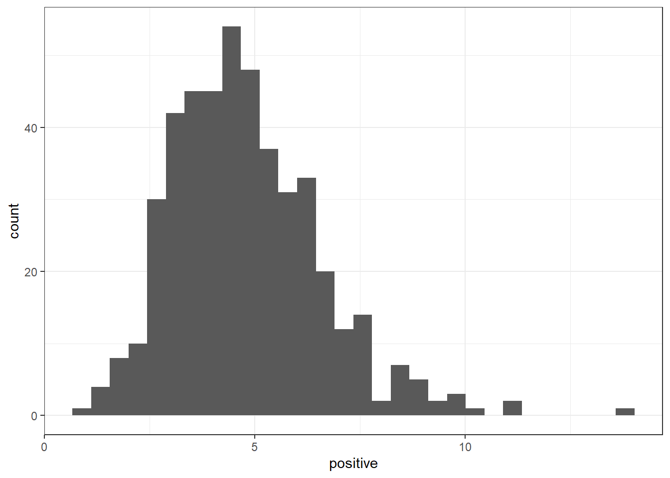
#Based on that, let's look at those that are out in the right tail (i.e., which are greater than 8, most positive)arlnow_covid_corpus[which(reviewSentiment_nrc$positive >8)]
Corpus consisting of 23 documents and 3 docvars.
text59 :
", Elementary-school-aged children will soon be able to get t..."

text65 :
", This sponsored column is by James Montana, Esq., Doran She..."

text89 :
"Members of Grace Community Church in Arlington honored thous..."

text123 :
", This column is written and sponsored by Arlington Arts/Arl..."

text135 :
", Peter’s Take is a weekly opinion column. The views and opi..."

text140 :
", Progressive Voice is a bi-weekly opinion column. The views..."

[ reached max_ndoc ... 17 more documents ]
Most terms seem to be around 3-7, and the highest is above 10.
Corpus consisting of 25 documents and 3 docvars.
text7 :
"Don’t look now but Covid cases are declining in Arlington., ..."

text53 :
"A post-Thanksgiving rise in Covid cases in Arlington appears..."

text124 :
", Progressive Voice is a bi-weekly opinion column. The views..."

text125 :
"Health Matters is a biweekly opinion column. The views expre..."

text127 :
", (Updated at 8:20 p.m.) The chairman of the Arlington GOP h..."

text141 :
", This is a sponsored column by attorneys John Berry and Kim..."

[ reached max_ndoc ... 19 more documents ]
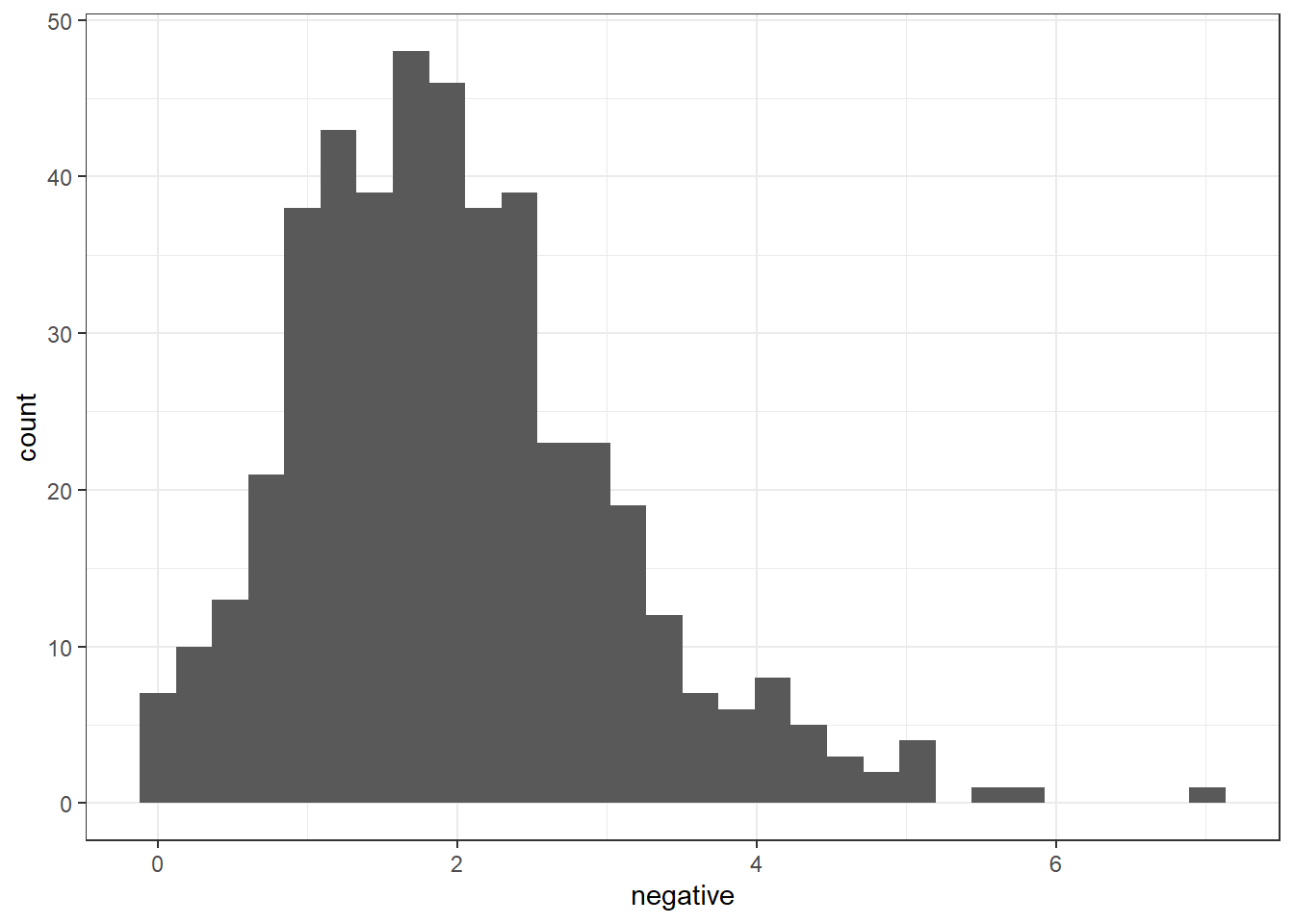
Most terms seem to be around 1-3, and the highest is above 6, and the lowest is 0.
These alone may not be the best indicators though, a combined measure may be better.
Corpus consisting of 29 documents and 3 docvars.
text2 :
"(Updated at 9:50 a.m.) Covid cases have held relatively stea..."

text7 :
"Don’t look now but Covid cases are declining in Arlington., ..."

text12 :
"The stock market drop aside, some other falling figures in A..."

text16 :
"Arlington County Board member Libby Garvey is quarantining i..."

text25 :
"For the last two months, Arlington County has been getting y..."

text37 :
"The average rate of new Covid cases in Arlington has fallen ..."

[ reached max_ndoc ... 23 more documents ]
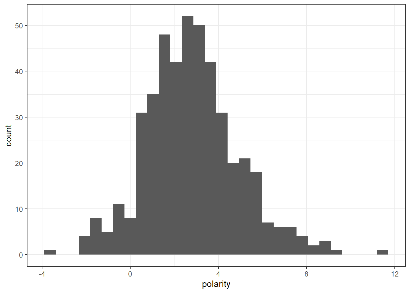
Most terms seem to be around 0-4, and the lowest close to -4 and the highest is almost 12.
Using Dictionaries with DFMs
For the dfm I am including most of the same preprocessing I did in the last post.
Code
# create a full dfm for comparisonarlnow_covid_dfm =tokens(arlnow_covid_corpus,remove_punct =TRUE,remove_symbols =TRUE,remove_numbers =TRUE) %>%dfm(tolower =TRUE) %>%dfm_remove(stopwords('english')) %>%dfm_remove(c("arlington", "county", "virginia", "$"))head(arlnow_covid_dfm, 10)
I think this is getting a little closer to what I can look at for my analysis. Looking at the emotions is interesting because things like anger, anticipation, disgust, fear, joy, negative, positive, sadness, surprise, trust, etc. Looking at the emotions of the text and seeing what most texts have over time can be really interesting and what I want to do for my next blog post.
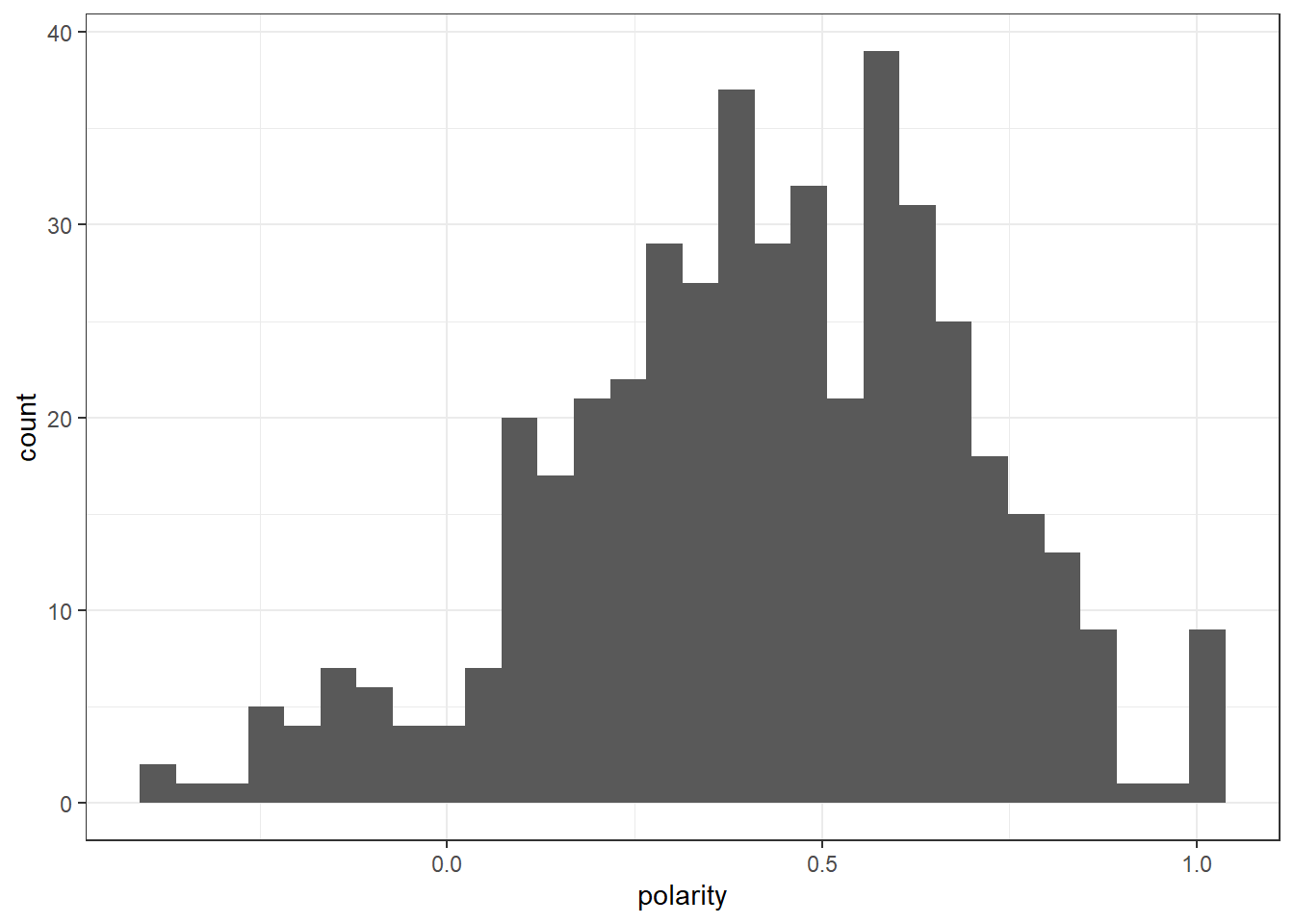
Next I’ll convert that to a data frame for further analysis, then create a polarity measure using the positive and negative measures.
Code
df_nrc =convert(arlnow_covid_dfm_nrc, to ="data.frame")names(df_nrc)
A lot of the polarity is centered around 0.5, although some reach 1 and a few go to 0 and below.
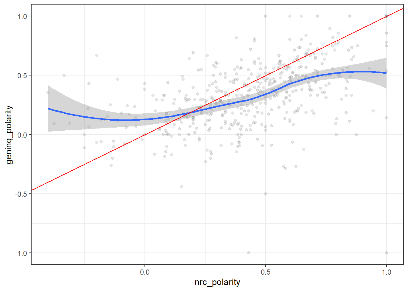
Dictionary Comparison
There are multiple dictionaries that can be used, so it may be helpful to compare them and how they work on this data.
Code
# convert corpus to DFM using the General Inquirer dictionaryarlnow_covid_dfm_geninq = arlnow_covid_dfm %>%dfm_lookup(data_dictionary_geninqposneg)head(arlnow_covid_dfm_geninq, 6)
I know that the dictionary used dependss on the analysis so I want to see this one too.
Code
# create polarity measure for geninqdf_geninq =convert(arlnow_covid_dfm_geninq, to ="data.frame")df_geninq$polarity = (df_geninq$positive - df_geninq$negative)/(df_geninq$positive + df_geninq$negative)df_geninq$polarity[which((df_geninq$positive + df_geninq$negative) ==0)] =0# look at first few rowshead(df_geninq)
The correlation of 0.45 is moderate, which is ok but not the best.
Apply Dictionary within Contexts
How is “vaccine” treated across the corpus of articles? Limit the corpus to just vaccine related tokens (vax_words) and the window they appear within.
Code
# tokenize corpustokens_LMRD =tokens(arlnow_covid_corpus, remove_punct =TRUE)# what are the context (target) words or phrasesvax_words =c("vaccine", "vaccinate", "vaccinated", "vax", "shot", "dose", "booster")# retain only our tokens and their contexttokens_vax =tokens_keep(tokens_LMRD, pattern =phrase(vax_words), window =40)
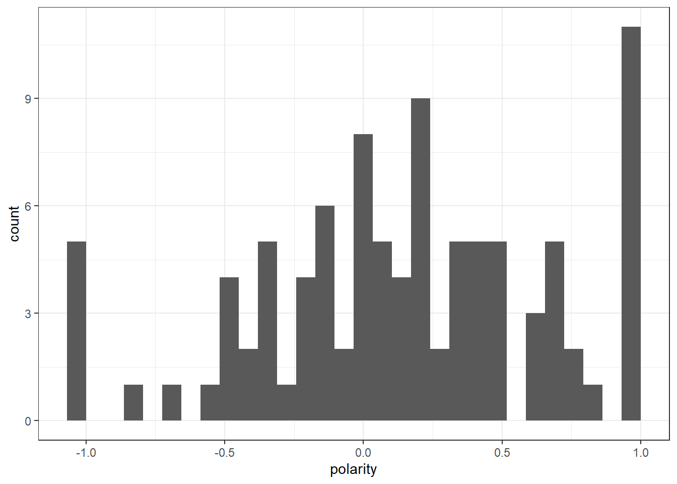
Pull out the positive and negative dictionaries and look for those within our token sets.
Drop articles that did not feature any emotionally valence words from the analysis, then take a look at the distribution.
Code
# convert to data framemat_vax =convert(dfm_vax, to ="data.frame")# drop if both features are 0mat_vax = mat_vax[-which((mat_vax$negative + mat_vax$positive)==0), ]# print a little summary infopaste("We have ", nrow(mat_vax), " reviews that mention positive or negative words in the context of vaccine terms.", sep ="")
[1] "We have 97 reviews that mention positive or negative words in the context of vaccine terms."
I kept this very general because I wasn’t sure how/if I should make my own dictionary (scheduled office hours to discuss and will update). I think I still want to keep working on some past suggestions like including another news source and looking at how specific words are connected and used (I did focus on vaccine and similar words here), but I haven’t included them yet as I don’t know exactly what I want to do with it.
Source Code
---title: "Blog Post 4 (Arlnow covid articles)"author: "Miranda Manka"desription: "Working with data - Dictionaries"date: "10/28/2022"format: html: toc: true code-fold: true code-copy: true code-tools: truecategories: - Miranda Manka---```{r}#| label: setup#| warning: false#| message: falselibrary(tidyverse)library(quanteda)library(quanteda.textplots)library(tidytext)library(plyr)library(ggplot2)library(devtools)devtools::install_github("kbenoit/quanteda.dictionaries")library(quanteda.dictionaries)remotes::install_github("quanteda/quanteda.sentiment")library(quanteda.sentiment)knitr::opts_chunk$set(echo =TRUE, warning =FALSE, message =FALSE)```## DataThe dataset contains 550 different articles from Arlnow (local news site in Northern Virginia) from March 2020 to September 2022. I decided to go back to March because that is when covid was officially declared a pandemic in the U.S. I may scrape more to get the months before March. I may also try to find a similar site for another county/city in another state to compare the two and see similarities and differences. Here I am just reading in the data from the csv I created and dropping the extra column that was created in the write.csv and renaming a column. I also removed articles where the title had "Morning Notes" as they weren't really articles but more recaps.```{r}arlnow_covid =read_csv("_data/arlnow_covid_posts.csv", col_names =TRUE, show_col_types =FALSE)arlnow_covid =subset(arlnow_covid, select =-c(1))arlnow_covid = dplyr::rename(arlnow_covid, text_field = raw_text)arlnow_covid = arlnow_covid[!grepl("Morning Notes", arlnow_covid$header_text), ]```## AnalysisMost of this analysis follows the week 8 tutorial we were given, I found it very helpful and I wanted to note where a lot of the code/information came from as I use a lot of it for this post.```{r}arlnow_covid_corpus =corpus(arlnow_covid, docid_field ="doc_id", text_field ="text_field")arlnow_covid_summary =summary(arlnow_covid_corpus)arlnow_covid_corpus_tokens =tokens(arlnow_covid_corpus, remove_punct = T)```### Dictionary AnalysisThe basic idea with a dictionary analysis is to identify a set of words that connect to a certain concept, and to count the frequency of that set of words within a document. The liwcalike() function takes a corpus or character vector and carries out an analysis–based on a provide dictionary–that mimics the software LIWC (Linguistic Inquiry and Word Count). The LIWC software calculates the percentage of the document that reflects a host of different characteristics.```{r}# use liwcalike() to estimate sentiment using NRC dictionaryreviewSentiment_nrc =liwcalike(arlnow_covid_corpus, data_dictionary_NRC)names(reviewSentiment_nrc)```I think this could be interesting but I don't know how helpful it is for my own terms because I am not sure how well they apply to the ideas.Looking at the most positive.```{r}ggplot(reviewSentiment_nrc) +geom_histogram(aes(x = positive)) +theme_bw()#Based on that, let's look at those that are out in the right tail (i.e., which are greater than 8, most positive)arlnow_covid_corpus[which(reviewSentiment_nrc$positive >8)]```Most terms seem to be around 3-7, and the highest is above 10.Looking at the most negative.```{r}ggplot(reviewSentiment_nrc) +geom_histogram(aes(x = negative)) +theme_bw()arlnow_covid_corpus[which(reviewSentiment_nrc$negative >4)]```Most terms seem to be around 1-3, and the highest is above 6, and the lowest is 0.These alone may not be the best indicators though, a combined measure may be better.```{r}reviewSentiment_nrc$polarity = reviewSentiment_nrc$positive - reviewSentiment_nrc$negativeggplot(reviewSentiment_nrc) +geom_histogram(aes(polarity)) +theme_bw()arlnow_covid_corpus[which(reviewSentiment_nrc$polarity <0)]```Most terms seem to be around 0-4, and the lowest close to -4 and the highest is almost 12.### Using Dictionaries with DFMsFor the dfm I am including most of the same preprocessing I did in the last post.```{r}# create a full dfm for comparisonarlnow_covid_dfm =tokens(arlnow_covid_corpus,remove_punct =TRUE,remove_symbols =TRUE,remove_numbers =TRUE) %>%dfm(tolower =TRUE) %>%dfm_remove(stopwords('english')) %>%dfm_remove(c("arlington", "county", "virginia", "$"))head(arlnow_covid_dfm, 10)dim(arlnow_covid_dfm)# convert corpus to dfm using the dictionary NRCarlnow_covid_dfm_nrc = arlnow_covid_dfm %>%dfm_lookup(data_dictionary_NRC)dim(arlnow_covid_dfm_nrc)head(arlnow_covid_dfm_nrc, 10)class(arlnow_covid_dfm_nrc)```I think this is getting a little closer to what I can look at for my analysis. Looking at the emotions is interesting because things like anger, anticipation, disgust, fear, joy, negative, positive, sadness, surprise, trust, etc. Looking at the emotions of the text and seeing what most texts have over time can be really interesting and what I want to do for my next blog post.Next I'll convert that to a data frame for further analysis, then create a polarity measure using the positive and negative measures.```{r}df_nrc =convert(arlnow_covid_dfm_nrc, to ="data.frame")names(df_nrc)df_nrc$polarity = (df_nrc$positive - df_nrc$negative)/(df_nrc$positive + df_nrc$negative)df_nrc$polarity[(df_nrc$positive + df_nrc$negative) ==0] =0ggplot(df_nrc) +geom_histogram(aes(x = polarity)) +theme_bw()```A lot of the polarity is centered around 0.5, although some reach 1 and a few go to 0 and below.### Dictionary ComparisonThere are multiple dictionaries that can be used, so it may be helpful to compare them and how they work on this data.```{r}# convert corpus to DFM using the General Inquirer dictionaryarlnow_covid_dfm_geninq = arlnow_covid_dfm %>%dfm_lookup(data_dictionary_geninqposneg)head(arlnow_covid_dfm_geninq, 6)```I know that the dictionary used dependss on the analysis so I want to see this one too.```{r}# create polarity measure for geninqdf_geninq =convert(arlnow_covid_dfm_geninq, to ="data.frame")df_geninq$polarity = (df_geninq$positive - df_geninq$negative)/(df_geninq$positive + df_geninq$negative)df_geninq$polarity[which((df_geninq$positive + df_geninq$negative) ==0)] =0# look at first few rowshead(df_geninq)```Combine all of these into a single dataframe to see how well they match up.```{r}# create unique names for each data framecolnames(df_nrc) =paste("nrc", colnames(df_nrc), sep ="_")colnames(df_geninq) =paste("geninq", colnames(df_geninq), sep ="_")# now let's compare our estimatessent_df =merge(df_nrc, df_geninq, by.x ="nrc_doc_id", by.y ="geninq_doc_id")head(sent_df)```I think there are some differences between the measures of polarity for the nrc vs geninq based on the measure.How well different measures of polarity agree across the different approaches.```{r}cor(sent_df$nrc_polarity, sent_df$geninq_polarity)ggplot(sent_df, mapping =aes(x = nrc_polarity,y = geninq_polarity)) +geom_point(alpha =0.1) +geom_smooth() +geom_abline(intercept =0, slope =1, color ="red") +theme_bw()```The correlation of 0.45 is moderate, which is ok but not the best.### Apply Dictionary within ContextsHow is "vaccine" treated across the corpus of articles? Limit the corpus to just vaccine related tokens (vax_words) and the window they appear within.```{r}# tokenize corpustokens_LMRD =tokens(arlnow_covid_corpus, remove_punct =TRUE)# what are the context (target) words or phrasesvax_words =c("vaccine", "vaccinate", "vaccinated", "vax", "shot", "dose", "booster")# retain only our tokens and their contexttokens_vax =tokens_keep(tokens_LMRD, pattern =phrase(vax_words), window =40)```Pull out the positive and negative dictionaries and look for those within our token sets.```{r}data_dictionary_LSD2015_pos_neg = data_dictionary_LSD2015[1:2]tokens_vax_lsd =tokens_lookup(tokens_vax,dictionary = data_dictionary_LSD2015_pos_neg)```Convert this to a DFM.```{r}dfm_vax =dfm(tokens_vax_lsd)head(dfm_vax, 10)```Drop articles that did not feature any emotionally valence words from the analysis, then take a look at the distribution.```{r}# convert to data framemat_vax =convert(dfm_vax, to ="data.frame")# drop if both features are 0mat_vax = mat_vax[-which((mat_vax$negative + mat_vax$positive)==0), ]# print a little summary infopaste("We have ", nrow(mat_vax), " reviews that mention positive or negative words in the context of vaccine terms.", sep ="")# create polarity scoresmat_vax$polarity = (mat_vax$positive - mat_vax$negative)/(mat_vax$positive + mat_vax$negative)# summarysummary(mat_vax$polarity)# plotggplot(mat_vax) +geom_histogram(aes(x = polarity)) +theme_bw()```I kept this very general because I wasn't sure how/if I should make my own dictionary (scheduled office hours to discuss and will update). I think I still want to keep working on some past suggestions like including another news source and looking at how specific words are connected and used (I did focus on vaccine and similar words here), but I haven't included them yet as I don't know exactly what I want to do with it.